Non Linear Behaviour of the SRPP
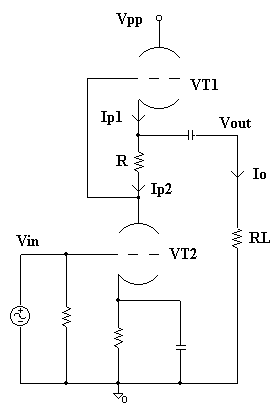
Fig. 1
The
SRPP circuit (acronym of Shunt
Regulated Push-Pull)
is known since the 50’s [1], [2] but it has gained his fame as “basic
block” for audio designs recently, at least in the west. Its use could be seen
as an intrinsic characteristics of the renewed interest of vacuum tubes applied
to the world of Hi-Fi reproduction. Oddly, this circuit is poorly used in the
pro-audio sector and solid-state designers ignore it altough proposed by Milmann and others [3]. Altough imperfect in its operation (as any amplifier
stage), the SRPP topology is able to mix good electrical performances with
semplicity of building and interesting sonic results. Since many characteristics
of this topology are not immediatly evident regarding to HCT point of view I
will dedicate wide space to analysis.
io=
ip1-ip2 (1).
Ref.
[4] contains a good explanation on the operation. The primary purpose of this
configuration was in the driving of low impedance loads, tipically “long”
cables terminated on low impedances (a
worry matter for the early television technique). The “tricks” consist in
varying the values of R or RL in order to alter the amplitude of ip1 and ip2
and, for the (1), to minimize the THD. By substituing the Small Signals
Equivalent Circuit (SSEC) to tubes
VT1 and VT2 in Fig. 1 the above condition it’s obtained when:
R=
1/gm + 2*RL/m
(2)
RL=
m*(R*gm
– 1)/2*gm
with
obvious meaning of symbols. Unfortunately a more deepened analysis that includes
non linear effects reduces the precision of (2). The main observation is that
both formulae furnish the solution to a non linear problem starting from a
linear presupposition (the SSEC hypothesis). In fact the upper triode receives
an input signal already corrupt in its harmonic content by the lower tube and
therefore the minimun in the THD not necessarily is obtained by differentiating
two currents with the same amplitude although out-of-phase; a similar mechanism
happened in Cascade Stages. The problematic is better understood with a Spice
simulation. If the circuit in Fig. 1 has the following charecteristics:
VT1=VT2=6SN7;
Vin=4Vpp e Rcath=1k, (3)
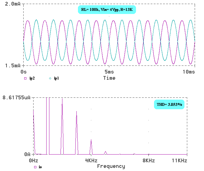
Fig. 2
in
the condition of greather symmetry for ip1 and ip2, io presents a THD of 3.053%
and R take a value very close to the first of the 2. The harmonic spectrum is
decreasing with the frequency, Fig.2. In the Fig. 3 you have the best condition
for the harmonic distortion, THD=0.5% and R=8K. You can see that ip1 and ip2
don’t result equal at all and the spectrum presents a 3rd harmonic
with position of dominion respect to the others.
A very important characteristic of SRPP derived directly from (1) but not easily comprehensible in a intuitve way consists in the ability to alter the phase relationship between ip1 and ip2 by varying R or RL. Fig. 4 shows the result of a Spice simulation of the circuit in Fig. 1 (with the istances 3) when R is varying between 4k and 10k by steps of 500W. Apart an obvious bias alteration, ip1, the current passing through the upper tube, is subjected to a phase inversion when R becomes elevated. Likewise, by varying RL between 5k and 100k by steps of 5k with R fixed you obtain the results of Fig. 5. For high load resistors ip1 and ip2 are in-phase, while the same becomes out-of-phase for low ones.
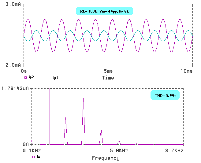
Fig. 3
From
here it emerges that utmost
potentialities of SRPP, as a shunt type push-pull, are obtained when, by varying
R or RL, ip1 and ip2 are out-of-phase. This peculiarity of SRPP circuit was well
understood from his inventor; unfortunetely now, in the majority of the cases,
we use it like a kind of common cathode amplifier with an active load and a low
output impedance.
The examen of the precedent simulations light up a fairly “curious” aspect: from Fig. 3 and 4 a value for R or RL exists that nulls ip1 current (remember ip1 and ip2 are dynamic variations) since a phase inversion is concerned. In these conditions the upper triode doesn’t influence the elaboration of the information that virtually will follow the path underlined in Fig. 6. This behaviour give us a wide margin in the choice of the upper device because, when ip1=0, it doesn’t compete for sonic texture. For example you could experiment with pentodes or j-fet as upper device and Direct Heating Triodes as lower device.
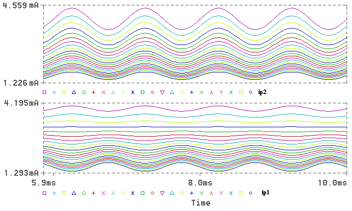
Fig.
4
A
better understanding of R’s or RL’s role can be obtained with a non linear
analysis of Fig. 1. Since:
ip1=
h1*eg1 + h2*eg12
(4)
ip2
= g1*Vin + g2*Vin2
(5)
eg1
= -Rip2
(6)
After
a bit of algebraic calculi you obtain the following expression:
io=ip1-ip2=
a*Vin4 + b*Vin3 + c*Vin2 +d*Vin
(7)
where:
a=
g2^2 * h2 * R^2
b=
2* g1*g2*h2
c=
g1^2*h2*R^2 – g2*(h1*R-1)
d=
-(g1*h1*R+g1)
(8)
and
for the (6):
io= Co + C1*sinwt + C2*cos2wt + C3*sin3wt +C4*cos4wt (9)
where:
Co=
3/8*g2^2*h2*R^2*Vp^4
+ ½*Vp^2*(g1^2*h2*R^2-g2*h1*R-g2);
C1=
-Vp*(g1*h1*R + g1);
C2=
-1/2*g2^2*h2*R^2*Vp^4 –1/2*Vp^2(g1^2*h2*R^2-g2*h1*R-g2);
C3=
-1/2*g1*g2*h2*R^2*Vp^3;
C4=
1/8*g2^2*h2*R^2*Vp^4;
(10)
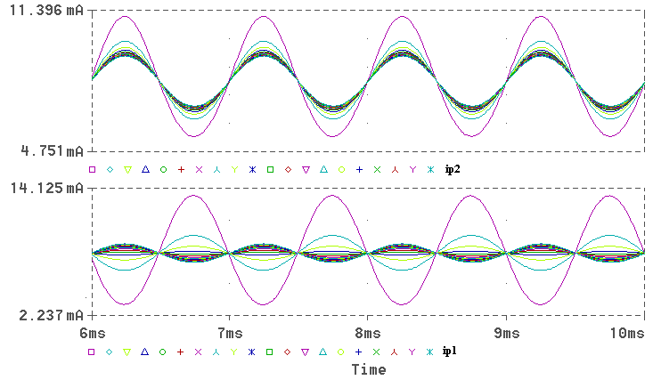
Fig. 5
The
main problem consist in the correct determination of [gi]
and [hi] coefficients. Such terms
could be determined after a characterization of the Mutual Dynamic
Characteristics (MDCs). You can
follow an analytical or numerical way.
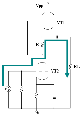
Fig. 6
Clearly,
the latter (that include also the experimental approach) leads to
faster results since to use a “curve
fitting” less informations are requested
for the tube characterization. Fig. 7 shows the DC loadlines of a
6SN7’s SRPP powered by 500Vcc source and Fig. 8 their MDCs rispectively
evalued by PSpice. Please observe the difficulty to deduce MDCs from loadlines
because you cannot extract from here the true phase relationship between ip1 and
ip2 currents. A curve fitting based
on the numerical values in Fig. 8 allow us to determine [gi]
and [hi] coefficients and therefore
to appraise partially the goodness of (10s), Table 1.
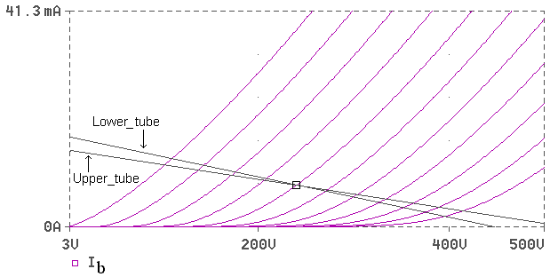
Fig.
7
Tab.
1
|
|
||
|
Amplitude
(Vp) |
2nd
Harmonic Calculated (V) |
2nd
Harmonic Pspice Evaluated
(V) |
|
1 |
6.422e-7 |
6.210e-7 |
|
2 |
2.569e-6 |
2.507e-6 |
|
3 |
5.759e-6 |
5.647e-6 |
|
4 |
1.027e-5 |
1.002e-5 |
|
5 |
1.605e-5 |
1.561e-5 |
|
6 |
2.310e-5 |
2.238e-5 |
|
7 |
3.144e-5 |
3.029e-5 |
|
8 |
4.100e-5 |
3.927e-5 |
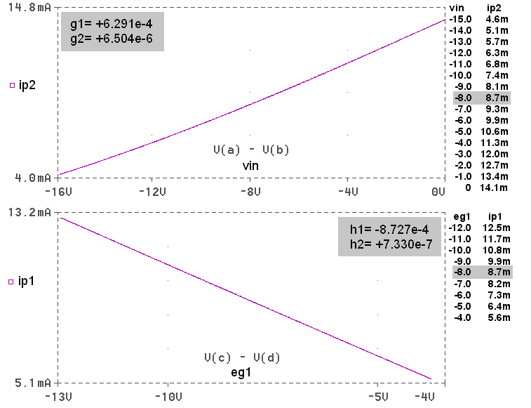
Fig.
8
Unfortunately mathematical expressions don’t have a large utility to correctly determine R or RL values because a lot of physical effects are keep out from (10’s). However the C2 expression in the (10’s) permits to intuit that a value in R or RL exists in order to minimize this coefficient therefore you can entrust the “crunch numbers” task to the electronic simulator or to the benchmark to directly determine the resistive values. I have easily characterized the SRPP behaviour with a set of simulations summarized in Figs 9-12 for input signals of 0.2Vpp, 2Vpp, 4Vpp, 6Vpp rispectively. On the graphics the X-axis always represents R values while Y-axis can have 1st, 2nd, 3rd, 4th harmonics and THD of output current.
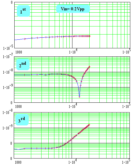

Fig. 9
Since the gain of a 6SN7’s SRPP is about 20dB you could think the first graphic set in Fig. 9 as referred to a line preamplifier, the sets of Figs 10 and 11 could represent the behaviour of gain stages in power amplifiers and finally the set in Fig. 12 could be the behaviour of a driver for power amplifiers.
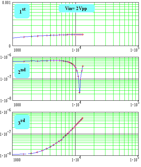
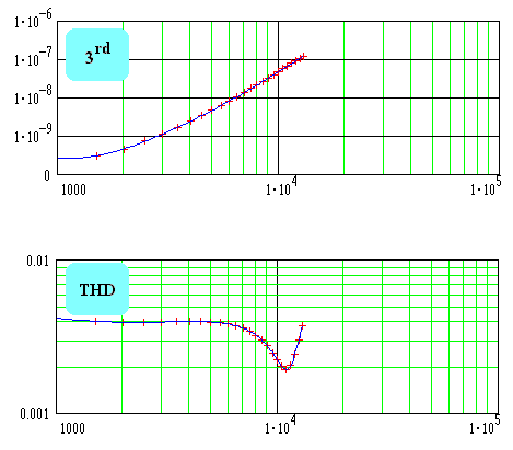
Fig. 10
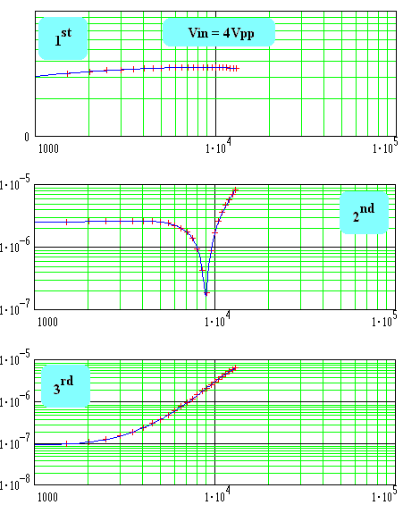
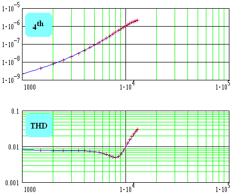
Fig. 11
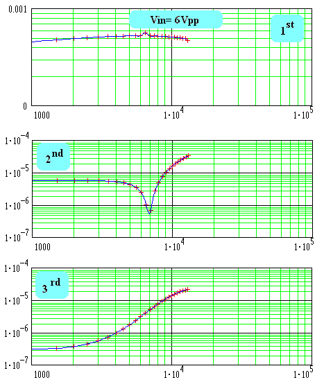
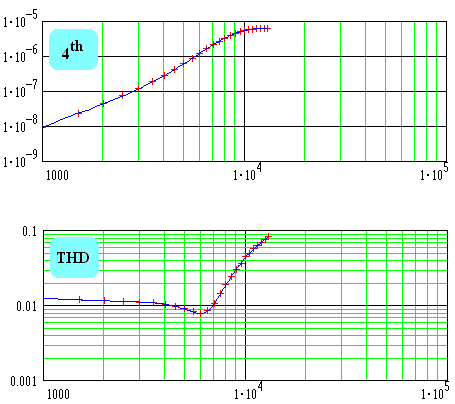
Fig. 12
All
graphics always show a minimum in the THD. When this minimum is reached, an
ulterior increment in R produces an abrupt THD surge. You can see from the
graphs that the optimal value in the THD is given when an opportune (dise-)equilibrium
between 2nd, 3rd
and 4th harmonics exists. 2nd harmonic is the
spectral component with a greater weight since its trend is similar to THD. The
2nd harmonic reduction is counterbalanced by a growth in the 3rd
harmonic. The increase in the 3rd harmonic involves, when this is
followed by a reduction in 2nd harmonic, a better simmetry of output
signal respect to Y-axis. Besides all graphs show a left-shift, for the R values
producing the minimum in the THD, when the input signals increase, Tab.2.
|
|
|
Input
Signal |
R
values for minimun in THD |
|
0.2Vpp |
13kW |
|
2Vpp |
11kW |
|
4Vpp |
9kW |
|
6Vpp |
7kW |
The fundamental presents a tendency weakly increasing with R in Figg. 9-10, while in Figg. 11-12 it presents even a maximum. Since by varying the R or RL values you can alterate the harmonic spectra of the signals, this metodology could be used to change the timbric imprint of the produced sound.
References:
| (1) | A. Peterson, D.B. Sinclair | A Single Ended Push-Pull Audio Amplifier, Proc. IRE, Vol.40, pp. 7-11, Jan 1952 |
| (2) | Yeh Chai | Analisys of a Single Ended Push-Pull Audio Amplifier, Proc. IRE, Vol. 11, pp.743-47, June 1953 |
| (3) | J. Millman and C.C. Halkias | Integrated Electronics, McGraw-Hill, New York, Appendix C, Problems 10.22, 10.23, 1972 |
| (4) | J. Milmann and H. Taub | Pulse, Digital and Switching Waveforms, McGraw-Hill, New York, Par. 3.17, 1965 |
|
What did you
think of this article? |