

|
|
|
|
|
Chapter 6 |
In the previous chapter some tests are carried on the values of the WCF, some results are obtained and some conclusion concerning them are drawn. Based on these conclusions, in this chapter two possible simple ways to compress the image are explored, considering the particular features of the wavelet coefficients belonging to the detailed groups, or the enormous quantity of almost insignificant coefficients.

Figure 5.1 : Order of setting to zero of the various subband of the wavelet coefficient matrix.
![]()
![]()
A first easy way to compress the image could be to remove progressively the information that every subband contains; this information represents the details, the edges and sometimes even the noise of the image, depending on subband and level.
5.1.1. EXPLANATION OF THE TESTS
The information carried by the wavelet coefficients belonging to a subband could be removed simply by setting to zero all the coefficients of that subband; the higher the number of the subbands cancelled, the lower will be the quality of the restored image, given that every time information is decreased a part is lost, but a higher compression ratio can be achieved. This idea is at the basis of the tests developed and of the results analysed in this chapter; after the DWT the appearance of the wavelet coefficient matrices will be changed gradually, replacing areas that represent various subbands with zeroes. The beginning of this replacing with the subband HH of the first level is done continuing until the subband LH of the third level; in detail the diagram in Figure 5.1 that represents the subbands in inverse order of importance for the quality of the restored image and the quantity of the information carried will be followed.
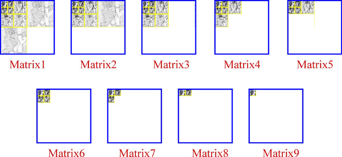
Figure 5.2 : Nine different WCF matrices obtained from the WCF original matrix by setting to zero various subbands.
| WCF Matrix | Matrix1 | Matrix2 | Matrix3 | Matrix4 | Matrix5 | Matrix6 | Matrix7 | Matrix8 | Matrix9 |
| Reconstructed
Image |
Imrec1 | Imrec2 | Imrec3 | Imrec4 | Imrec5 | Imrec6 | Imrec7 | Imrec8 | Imrec9 |
| E. C. R. | 1.28: 1 | 1.78: 1 | 2.91: 1 | 3.46: 1 | 4.27: 1 | 5.56: 1 | 6.02: 1 | 6.56: 1 | 7.21: 1 |
| # WCF used | 196608 | 131072 | 65536 | 49152 | 32768 | 16384 | 12288 | 8192 | 4096 |
| % WCF used | 75 | 50 | 25 | 18.75 | 12.5 | 6.25 | 4.69 | 3.13 | 1.56 |
Table 5.1 : Correspondence between WCF matrix, image reconstructed, Equivalent Compression Ratio, Number and Percentage of WCF for each of the19 WCF matrices used.
In this way at the end of the whole process 9 different matrices, shown in Figure 5.2 and called MatrixX , are obtained; there will be an increasing number of zeroes and a decreasing number of significant coefficients inside. Each of these matrices is used as a wavelet coefficients matrix obtaining, by means of an IDWT operation, 9 different images of decreasing quality, called ImrecX . In this tests we are interested in the values of the PSNR which are obtained for every image; it is also possible to have a little idea about a possible compression ratio associated with each of the 9 images.
A simple way to think about a possible compression ratio, and so to give a number to make comparison, is to use 8 bits for the WCF considered significant in the tests and that left unchanged, and 1 bit only for the WCF set to zero; in this way it is possible to calculate the various E. C. R. shown in Table 5.1. These values are useful to just give a rough idea, because it is obvious that other methods should be used to code and compress the remaining coefficients further. Comparing the quality of these images with the real image quality by the use of the PSNR values some interesting results that show the quantity and quality of the information carried by the wavelet coefficients of a particular subband are obtained.
.......cut.........
![]()
![]()
Up to now only few comparisons between the results
obtained using different QMF are shown; another important result obtained
from these tests is the comparison, for every QMF used, between the different
images, or a critical evaluation of the change of the PSNR values between
close images. This comparison is possible looking at the differences between
the PSNR values as they are shown in Table 5.3 for the Bio CDF 3.9; in
this Table the Gap shows the difference of the PSNR values between two
adjacent images (ImrecX and ImrecX+1). In the Table 5.3 are shown the
values with respect to the Bio CDF 3.9 QMF because these QMF results are
the best, even if the same values with only a few differences are found
within all the different QMF used. A first interesting indication on how
the Wavelet Coefficients are important is shown on the first 2 values of
the parameter Gap; actually setting to zero the WCF of the subband I and
L (Matrix2 and Matrix1), a significant decrement of the PSNR, 4.9 and
2.5 is depicted.
| Imrec1 | Imrec2 | Imrec3 | Imrec4 | Imrec5 | Imrec6 | Imrec7 | Imrec8 | Imrec9 | |
| PSNR | 43.35 | 38.45 | 35.92 | 35.24 | 33.87 | 32.75 | 32.14 | 31.04 | 30.08 |
| Gap | - | 4.90 | 2.53 | 0.68 | 1.37 | 1.12 | 1.61 | 1.10 | 0.96 |
Table 5.3 : PSNR and Gap values for the Bio CDF 3.9.
These first two numbers show how much the wavelet coefficients of the first two subbands are important maintaining a high level of quality; this happens even if they have values that are only 1-2 percent as regard as the maximum value of WCF and even if they are only a little part of the whole WCF of the subband. The third value of the parameter Gap shows how the removal of the diagonal subband of the second level (Matrix2) does not affect too much the quality of the image, this is because there is a small number of significant coefficients, they are low in value and they are actually not so important for maintaining the quality at this level of less information. The other values of the Gap between PSNR values of adjacent images are more or less about 1-1.5 dB and this shows a constant loss of quality every time a subband is removed.
.......cut.........
![]()
![]()
5.2. WAVELET COEFFICIENTS THRESHOLDING
5.2.1. EXPLANATION OF THE MEANING OF THE TESTS
In the previous section a first step to reduce the amount of WCF needed to build, through a IDWT, a decompressed image is analysed; the big problem in that method is the leaving of a lot of insignificant coefficients in the subband unchanged and the removing of some significant coefficients from the subband set to zero. In this section it is depicted another way to compress or reduce the amount of WCF important for the IDWT; in this simple method all the WCF that have values lower than a threshold value, are set to zero, considering them as insignificant, and leave unchanged the coefficients with values bigger than the threshold values. With this method no distinction is made if the WCF belongs to a particular subband, but only if its value is big enough to be significant; a future improvement of this method could be to use different threshold values for different subbands, relating them to the maximum values of their subbands. The choice of the threshold values in these tests is made basing on the totality of the WCF values; this is the algorithm followed:
.........cut.........
![]()
![]()
Our analysis of the result on the tests is begun with the values of the PSNR belonging to the Y component; in the Figure 5.7 a detail of the original image Ima3 is shown and the same detail for the other 10 reconstructed images obtained at different thresholds. Looking at the results in general it is possible to say that the threshold at 0.1 and 0.05 percent give images (Tima9 and Tima10) with a quality too low to be taken into consideration, in fact the values of PSNR are about 23.7-25.6 and 10.3-12.7 respectively. In these two cases 262 and 131 coefficients are really not enough to perform an acceptable IDWT, especially in the second case as the two images shown in Figure 5.7 show us. They are too blurred and the objects in them are not resolved sufficiently. For the other thresholds, as seen from Table 5.7 and Figure 5.7, after the IDWT, there are reconstructed images that, also with quality variable depending on the threshold, show however the features of the objects presented in the original images. Even if it is difficult to have a good resolution on the images printed on paper, until the threshold of 2 % (Tima5), the reconstructed images have good quality; the image at 1 % (Tima6) shows an acceptable quality whereas the images at 0.5 % and 0.3 % (Tima7 and Tima8) have some distortions in them that decrease their quality.

Figure 5.7 : Detailed parts of Ima3 captured from the original image and the 10 reconstruction images.
![]()
![]()
The results for each of the 5 images show that,
also with different values of PSNR, the trends within the various groups
and between each other, are the same as seen before; actually the best
QMF seen previously are the best for each image. With the help of Table
5.8, in which there are the values of the PSNR for the Symlet 4 QMF for
the 5 images, shown in Figure 4.5, and with the help of the Figure 5.9,
in which the same values are diagrammed, it is possible to see the trend
of the different curves. It is possible to notice that image Ima1 has
the lower values of PSNR, at least until 1 percent of the threshold; this
shows that Ima1 has a lot of significant WCF, even if they have low values.
| Tima1 | Tima2 | Tima3 | Tima4 | Tima5 | Tima6 | Tima7 | Tima8 | Tima9 | Tima10 | |
| Ima1 | 36.85 | 34.55 | 34.02 | 33.45 | 32.78 | 31.87 | 31.10 | 30.47 | 28.46 | 10.64 |
| Ima2 | 42.31 | 39.69 | 39.07 | 38.37 | 37.52 | 36.36 | 35.28 | 34.19 | 27.67 | 7.24 |
| Ima3 | 39.71 | 36.76 | 36.02 | 35.15 | 33.99 | 31.96 | 29.11 | 27.09 | 20.28 | 13.37 |
| Ima4 | 40.59 | 37.99 | 37.33 | 36.57 | 35.58 | 33.94 | 32.29 | 30.56 | 23.29 | 11.65 |
| Ima5 | 40.98 | 38.27 | 37.61 | 36.85 | 35.91 | 34.46 | 32.94 | 31.20 | 24.48 | 8.95 |
Table 5.8 : PSNR values for 10 reconstructed images, for 5 initial images and for Symlet 4.
Actually as seen in the previous section, this image contains a lot of quite small edges that give an high number of small but significant WCF. On the other side the image Ima2 has the highest values among the 5 images as in the previous section; this shows that the image contains a lot of insignificant coefficients that are set to zero without a big loss of quality, and only a small number of significant coefficients. 1 % of the WCF for this image are enough to have the same values of PSNR as 10 percent of WCF for the image Ima1. The other 3 images have values that are near to the mean values previously seen, Ima3 nearer to Ima1 and Ima4 and Ima5 nearer to Ima2; all the 5 curves have however more or less the same trend: the value of PSNR decreases with the decrement of the threshold, as noticed from the Figure 5.9, at least until the values of 1 percent; after that threshold every image has its own history, depending on how much the group of the higher values of WCF are important for the reconstruction of the image.
Looking at the original high definition, 3710 ´ 2440 size, image, from which we take all the test images, and setting to zero the WCF as in this test, it is possible to notice that, improving the compression, the first group of significant WCF removed are the WCF belonging to the background object, that are not particularly interesting for the purposes; for that reason even if the wavelet coefficient removing is high, the quality of the interesting objects remains good.
![]()
![]()
Looking at the results of the tests made on the Cb and Cr components, with the help of Table 5.9, even with different values of PSNR the trends found for the Y component are respected by the Cb and Cr components concerning the different QMF within the families and among them. As an example of these values a comparison among the values of the results obtained for the components Y, Cb and Cr with the QMF Symlet 4 is done; these values shown in Table 5.9 and in Figure 5.9, indicate to that they decrease more or less in the same way even if for the component Cb and Cr they are higher compared with the values of the Y component. This values are 3.3 dB and 1.6-2 dB higher respectively for the high values of threshold, 10 % and 5 % and with the decreasing of the percentage of the threshold this gap increase up to 4 dB and 3 dB respectively for 1 % of the threshold.
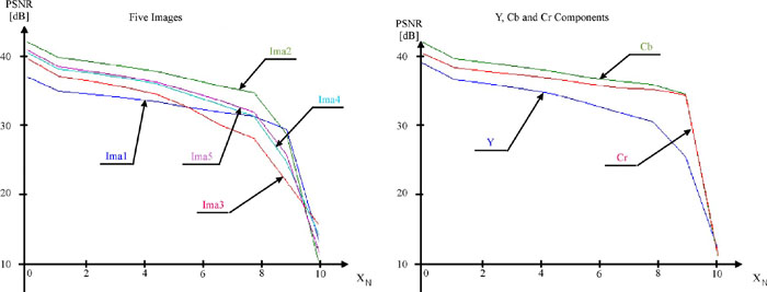
Figure 5.9 : PSNR values of the 10 different reconstructed images for the 5 initial images (left) and 3 components Y, Cb and Cr (right) for Symlet 4 QMF.
These features show that a lower number of significant
coefficients are lost when the threshold is high, 5-10 %, actually the
remaining part of the coefficients are more significant for Cb and Cr components.
The importance of this small group of significant coefficients becomes
more and more noticeable with the decreasing of the threshold for the Cb
and Cr components than for the Y component, so it is possible to compress
better these two components using for them less bits and leaving a large
part of the bit allocation for the Y component. An example of these could
be, following the values on the Table 5.9, trying to reach the goal of
a quality of about 37.5 dB for each component, a quality which is more
than acceptable as seen before. For the Y component we have to use 5 %
of the WCF, 13107 coefficients, for the Cr component 2 %, 5243 coefficients
and for the component Cb 0.9 %, 2359 coefficients; this means that 63.3
% of the total number of bits have to be used to code the Y component,
25.3 % for the Cr and 11.4 % for the Cb.
| Tima1 | Tima2 | Tima3 | Tima4 | Tima5 | Tima6 | Tima7 | Tima8 | Tima9 | Tima10 | |
| Y | 40.09 | 37.45 | 36.81 | 36.08 | 35.16 | 33.73 | 32.16 | 30.73 | 25.08 | 10.41 |
| Cb | 43.41 | 40.71 | 40.10 | 39.45 | 38.71 | 37.78 | 37.12 | 36.69 | 35.13 | 9.12 |
| Cr | 41.73 | 39.30 | 38.76 | 38.19 | 37.54 | 36.75 | 36.21 | 35.88 | 35.02 | 9.51 |
Table 5.9 : PSNR values for 10 reconstructed images, for Y, Cb and Cr components and for Symlet 4.
In reality a high quality for the component Y is achieved, because the luminance is often more important than the colour. So the gap between the bits used by the 3 components could increase in favour of the Y component; for example a quality of 40 dB for Y and 37.5 for Cb and Cr give 77.5 % of bits for Y component and 15.5% and 7 % for Cr and Cb components respectively. In the first case it is possible to reach an E.C.R. of 38 : 1 and in the second case of 23.3 : 1. As seen before the quality of the image is more than acceptable even if values of PSNR for the Y component of 36-37 dB are reached; in this case it is possible to reduce the values of PSNR reached by the Cb and Cr component down to 35-36 dB maintaining a good level of total quality. Quantifying this, we can use 4 % of WCF for the Y and only 0.2 % for Cb and Cr, using 90.9 % bit for Y, and 4.55 % bit for each Cb and Cr component; making a comparison with the total number of WCF used and using the same process for counting the compression ratio the high E.C.R. of 68.2 : 1 could be reached, remembering that this is only a rough number that could be increased with further kind of coding.
![]()
![]()
In the two previous chapters the results on the tests developed with the purpose of setting to zero some WCF, consider insignificant, are discussed, and the quality of the reconstructed image obtained is compared by the PSNR values; the tests are developed varying the range of the different QMF families, the component Y, Cb and Cr and the images used. In this chapter some conclusions from these results are drawn, to have a better idea about which could be the different QMF to use within different coding algorithms and which feature are in the different parts or objects of the images to compress. A result of the test is to recognise within a subband what wavelet coefficients are the insignificant; then try to set to zero, or roughly quantize them. This can be done by the threshold technique, and by some algorithm like Shapiros EZW and Said & Pearlmans SPIHT algorithms analysed in a following chapter. The threshold technique is more focused on this point than the first technique analysed, that sets to zero the subbands independently from their WCF values. In both techniques it is possible to notice that apart from some QMF, all the results obtained show that the differences between the PSNR values obtained using different QMF is not really high, and this is a confirmation that almost all the different QMF are very useful to use to compress the images to a high level; among the various QMF however there are some that allow to reach a better result. These QMF are the best almost every times, independently of the images to compress and of the 3 components, Y, Cb and Cr. Comparing the results of the 2 techniques two different trends with the range of the QMF within the various families are shown, in fact in the first technique the increasing of the range carries an increment of the PSNR values, whereas in the second technique a decrement of the values is noticed.
Between the different families, the orthogonals are almost all the time better than the biorthogonals, only the Bio CDF 3.x is at the same level in the first techniques. The most interesting QMF, as seen in the threshold technique section, are Sym 4, Sym 6, Sym 8, Daub 4, Daub 6 and Coif 1, whereas the Bio CDF 2.4 and Bio CDF 2.2 begin to become really interesting at high threshold values (high compression ratios). An important feature of the image to compress is that the object with strong edges, many changes of luminance or colour, interesting from the point of view of the maintenance of a high level of quality, have a small number of WCF with high values and usually placed in second and third level. The object with a lot of little scattered edges like the background, sand or pebbles, have instead a lot of WCF with values not too small, usually in the first and second level. For every image and for every QMF, and also with every compression technique it is possible to find that the components Cb and Cr have less significant WFC than the Y component, in fact with the same number of WCF removed the quality is better and the PSNR is higher; for this reason fewer bits are used to code the Cb and Cr components and reach a higher compression ratio, maintaining the same quality. Another result obtained is the consideration that between the three detailed subbands at every level the diagonal subband has coefficients more insignificant than the horizontal and vertical subbands; in this way ii is possible to concentrate more on these two subbands to maintain a high level of quality of the images.
![]()
![]()
E-mail to:
eug67@supereva.it![]() e.ballini@eng.abdn.ac.uk
e.ballini@eng.abdn.ac.uk![]()