Sono trascorsi molti anni da quella conferenza. Non molto tempo dopo, a causa di un'esperienza traumatica, egli abbandonò la ricerca. Solo di recente è tornato ad interessarsi di fisica ed ha fatto le scoperte che pubblica in questo sito. Nella trattazione egli ha evitato l'uso di matematiche sofisticate, in modo da rendere il materiale comprensibile anche da persone che non possiedono titoli di studio universitari. Per tale motivo, a volte i concetti possono apparire triviali ad un lettore esperto, ma l'autore indugia su di essi a beneficio di coloro che non hanno familiarità con tali teorie fisiche e per renderle quindi comprensibili al maggior numero di persone possibile. Infatti, le nuove scoperte riguardano argomenti che solleticano la fantasia e possono essere apprezzate anche da chi non è dedicato alla scienza fisica. Esse sono precedute da teorie e fatti già accettati, allo scopo di fornire una base di conoscenze minime necessarie alla corretta comprensione dei fenomeni descritti. Per esempio, la nuova teoria sull'etere e sull'inerzia è preceduta dalla teoria della relatività speciale e da altri argomenti ad essa attinenti, la teoria del tempo guida e l'originale descrizione dell'effetto Compton da alcune informazioni di meccanica quantistica.

Se riconosciute corrette, le scoperte presentate sono molto importanti, in quanto danno risposta a domande che hanno assillato gli scienziati per molti decenni. Esse inoltre aprono la strada a nuove ricerche e a nuovi modi di comprendere l'universo in cui viviamo.

Several years have passed since that conference. Not long after that, because of a traumatic experience, he abandoned research. Only in the past few years he came back to physics and made the discoveries that are published in this site. In describing the material he has avoided the use of sophisticated maths, in order to make it comprehensible also to people that don't possess a university degree. For that reason, sometimes the concepts may appear trivial to an experienced reader, but the author abounds in explaining them for the sake of those who aren't familiar with such physical theories and in order to make them palatable to as many people as possible. In fact, the new discoveries regard matters that excite the fantasy and may be appreciated even by people that aren't dedicated to the physical science. They're preceded by well-accepted theories in order to give a minimum base knowledge necessary for gaining the right comprehension of the discussed phenomena. For example the new theory regarding the ether and inertia is preceded by the special theory of relativity and other related arguments, the leading time theory and the Compton effect by some quantum mechanical informations.

If recognized true, the discoveries presented here are very important, because they give an answer to questions that have puzzled scientists for several decades. They also open the way for new research and new ways of looking at the universe we live in.

Contenuto

Nota: L'asterisco denota una teoria sviluppata dall'autore

1. Introduzione alla relatività

2. La dilatazione del tempo

3. La contrazione dello spazio

4. La contemporaneità in relatività

5. Evidenze di modificazioni di spazio e di tempo

6. La trasformazione di Lorentz

7. La metrica di Minkowski

8. La teoria della relatività

9. La massa relativistica

10. Il significato della dilatazione del tempo (*)

11. Corrispondenza tra l'etere e l'universo fisico (*)

12. Proprietà dello spazio-tempo (*)

13. L'origine dell'inerzia (*)

14. Il principio di indeterminazione

15. Il momento angolare in meccanica quantistica

16. La direzione del tempo e il tempo guida (*)

17. Il processo Compton (*)

18. Ulteriori conseguenze della teoria del tempo guida (*)

19. L'enigma della corona solare (*)

Contents

Note: The asterisk denotes a theory devolped by the author

1. Introduction to relativity

2. The time dilation

3. The space contraction

4. Contemporaneity in relativity

5. Relativistic evidences

6. The Lorentz transformation

7. The Minkowski metric

8. The theory of relativity

9. The relativistic mass

10. The meaning of the time dilation (*)

11. Correspondence between the ether and the physical universe (*)

12. Space-time properties (*)

13. The origin of inertia (*)

14. The uncertainty principle

15. Angular momentum in quantum mechanics

16. The direction of time and the leading time (*)

17. The Compton process (*)

18. Further consequences of the leading time theory (*)

19. The coronal puzzle (*)

Introduzione alla relatività

Cominciamo la nostra considerazione della teoria della relatività cercando di ottenere le leggi che la governano. Forse sai che la teoria della relatività dice che le misure degli intervalli di spazio e di tempo dipendono dalla velocità con cui si muove chi le esegue. Infatti, considera questa semplice situazione: supponi che mentre stai camminando lungo una strada tu veda passare in auto un amico e ti chieda: “La durata tra due ticchettii del mio orologio durano quanto quelli dell'orologio del mio amico che sta viaggiando in auto?” Se fossi tu ad eseguire entrambe le misurazioni, cioè se la misurazione fosse fatta “nel tuo sistema di riferimento”, la risposta è no. Naturalmente, nel dire questo non sono prese in esame le imperfezioni degli orologi. In altre parole, mentre è vero che la differenza tra le due misure temporali è molto piccola e che nessun orologio ordinario è in grado di mostrarla, tuttavia i due orologi procedono con velocità diverse e la differenza non è dovuta a qualche loro imperfezione, ma alla fisica che ne è coinvolta.

Questa è solo teoria, potresti dire. No. In seguito considereremo esempi che mostreranno che la dilatazione dei tempi e la contrazione degli spazi sono reali e producono effetti osservabili. Essi mostreranno pure che l'alterazione del tempo e dello spazio non concerne solo orologi e metri, ma tutti i processi fisici in cui sono coinvolti spazio e tempo.

Riguardo ai due orologi appena considerati, quale dei due è più veloce e quale più lento? La straordinaria risposta è che ciò dipende dal punto di vista (dalla velocità dell'osservatore o del sistema di riferimento). Se tu fossi in grado di leggere il quadrante dell'orologio del tuo amico, noteresti che esso non procede con la stessa velocità del tuo (per chi è più esperto aggiungo che la differenza non è dovuta all'effetto Doppler). Viceversa, se il tuo amico potesse osservare il tuo orologio, egli noterebbe che è il tuo a procedere più lentamente! In conclusione, quale orologio vince la corsa? Nessuno dei due, ossia, dal tuo punto di vista, il tuo vince!

Prima di procedere ad un esperimento concettuale che ci permetta di calcolare la dipendenza degli intervalli temporali dalla velocità dell'osservatore, consideriamo l'esperimento che condusse Einstein a formulare la teoria della relatività. Era l'anno 1887 e alcuni scienziati si chiedevano quale fosse la velocità della terra rispetto all'etere. Infatti in quel tempo si pensava che l'intero universo fosse pervaso da una specie di sostanza, l'etere, un concetto originato dagli antichi greci e che è tuttora dibattuto. L'esperimento si basava sul seguente ragionamento: se l'etere esiste, allora 1) nel corso dell'anno la terra si muove con velocità diverse rispetto ad esso a motivo dell'orbita che essa compie attorno al sole, mentre 2) la luce si muove sempre con la stessa velocità rispetto all'etere, indipendentemente dalla velocità della terra o dell'osservatore. Questa è basilarmente l'idea. Di conseguenza, esaminata dalla terra la luce dovrebbe manifestare diverse velocità nel corso dell'anno e la loro misurazione dovrebbe permettere di determinare la velocità della terra rispetto all'etere.

Per comprendere meglio questo aspetto, chiamiamo v la velocità della terra e c quella della luce, entrambe rispetto all'etere, e cerchiamo di calcolare la velocità della luce dal punto di vista della terra. Un raggio di luce che si muova nella direzione di moto della terra dovrebbe possedere una velocità ridotta, pari a c – v. Similmente, nella direzione opposta dovrebbe apparire muoversi con velocità c + v. Quindi, misurando la velocità della luce in varie direzioni si dovrebbe essere in grado di determinare la velocità della terra rispetto all'etere. Infatti, supponi che dal punto di vista di chi sta sulla terra la velocità della luce lungo una certa direzione sia w, un po' più piccola di c. Questo significa che nella direzione del raggio di luce la velocità della terra è v = c – w, mentre se w è maggiore di c, allora la terra si muove in direzione opposta con velocità v = w – c. Perciò vediamo che, se le ipotesi riguardo all'etere sono corrette, misurando la velocità della luce lungo varie direzioni e mediante un semplice calcolo dovrebbe essere possibile ricavare la velocità della terra rispetto all'etere.

Nel 1887 sulla base di un ragionamento simile Michelson e Morley tentarono di determinare la velocità della terra rispetto all'etere tramite misure della velocità della luce. Il risultato fu sconvolgente! La velocità della luce era sempre la stessa in tutte le direzioni e durante tutto il corso dell'anno. Poiché la terra si muove alla velocità di circa 30 km/sec attorno al sole e d'altra parte l'esperimento era in grado di misurare velocità con precisione molto maggiore (5 km/sec), il risultato dimostrò al di là di ogni dubbio che la velocità della luce è sempre la stessa in ogni direzione.

Questo è il risultato fondamentale da cui è possibile giungere alla conclusione che gli intervalli di spazio e di tempo cambiano con la velocità dell'osservatore e ottenere le formule che mettono in relazione le lunghezze degli intervalli misurati da due osservatori in moto relativo.

Pagina principale

Introduction to relativity

Let's start our consideration of the theory of relativity by trying to derive some of the laws that govern it. Among other things, it's a known fact that according to the theory of relativity the measurements of the space and time intervals depend on the velocity of the observer. Just to make things clear, consider this simple situation: while you're walking on a street and observe the cars passing by, you see in one of them a friend of yours, and ask yourself: “Does the duration between two ticks on my clock last as long as those on my friend's clock, who is traveling in the car?” If both measurements are made by you, i.e. from the point of view of your system of reference, then the answer is no. Of course, in saying this we do not take into account the imperfections of the clocks. In other words, while it's true that the difference between the two time measurements is very small and that no ordinary clock is able to show it, the two clocks tick with different speeds, and the difference is not due to some imperfection, but to the physics involved.

This is just theory, one might say. No. Later on, we shall consider an example showing that the time dilation and space contraction are real and produce observable effects. It will also show that the alteration of time and space doesn't regard only clocks or measuring rods, but any physical process involving space and time.

Regarding the two clocks we just considered, which one moves faster and which one slower? The amazing thing is that it depends on the point of view (on the velocity of the observer, or of the system of reference). If you were able to read the quadrant of your friend's clock, you'd notice that it doesn't tick as fast as yours (for the experienced reader, I add that this difference isn't due to a Doppler effect). Viceversa, if your friend could observe your clock, he'd find that it's yours that runs slower! In conclusion, which clock wins the race? Neither one, or, from your point of view, yours wins!

Before proceeding to consider a conceptual experiment that allow us to calculate the time dependence of the time intervals on the velocity of the observer, let's consider the experiment that led Einstein to formulate the theory of relativity. It was the year 1887 and some scientists were asking what were the velocity of the earth with respect to the ether. In fact, at that time it was thought that the whole universe was pervaded by a sort of substance, the ether, a concept originated by the ancient Greeks that's still debated today. The experiment was based on this reasoning: if the ether exists, than 1) during the year the earth moves with varying velocities with respect to it, due to its orbit around the sun, while 2) light moves with a well defined, constant velocity with respect to the ether, independently from the earth's or the observer's velocity. This is basically the idea. Consequently, as seen from earth, light should exhibit varying velocities in the course of the year, and a measurement of its speed should permit to determine the earth's velocity with respect to the ether.

In order to better understand this aspect, let's call v the velocity of the earth, and c the velocity of light, both with respect to the ether, and try to calculate the speed of light measured from earth. The velocity of the light that moves in the direction of motion of the earth should appear reduced, and be equal to c – v. For a similar reason, on the opposite direction it should appear to be moving with velocity c + v. Hence, by measuring the speed of light along various directions, one should be able to determine the earth's speed v with respect to the ether. In fact, suppose that from the earth point of view the speed of light along a certain direction be w, a little slower than c. This means that in the direction of the light beam the earth's speed is v = c – w, while if w is greater than c, than the earth moves in the opposite direction, and its velocity is v = w – c. So, we see that if the hypotheses regarding the ether are true, by measuring the speed of light along various directions and through a simple calculation it should possible to derive the earth's velocity relative to the ether.

In 1887, driven by a reasoning like this, two physicists, Michelson and Morley, tried to determine the earth's velocity with respect to the ether by measuring the speed of light. The result was astonishing: the measured speed of light was the same along any direction all year round! Since the earth moves with a velocity of about 30 km/sec around the sun, while the experiment was able to detect velocities much smaller than that, the result proved beyond any doubt that the speed of light is always the same in any direction.

This is the fundamental result from which it's possible to get to the conclusion that the space and time intervals change with the velocity of the observer, and to obtain the formulas that relate the lengths of the intervals measured by two observers in relative constant motion.

Home

La dilatazione del tempo

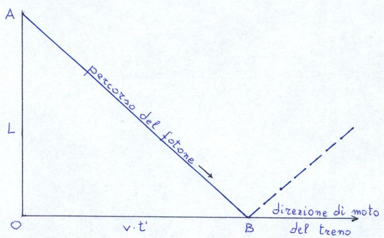
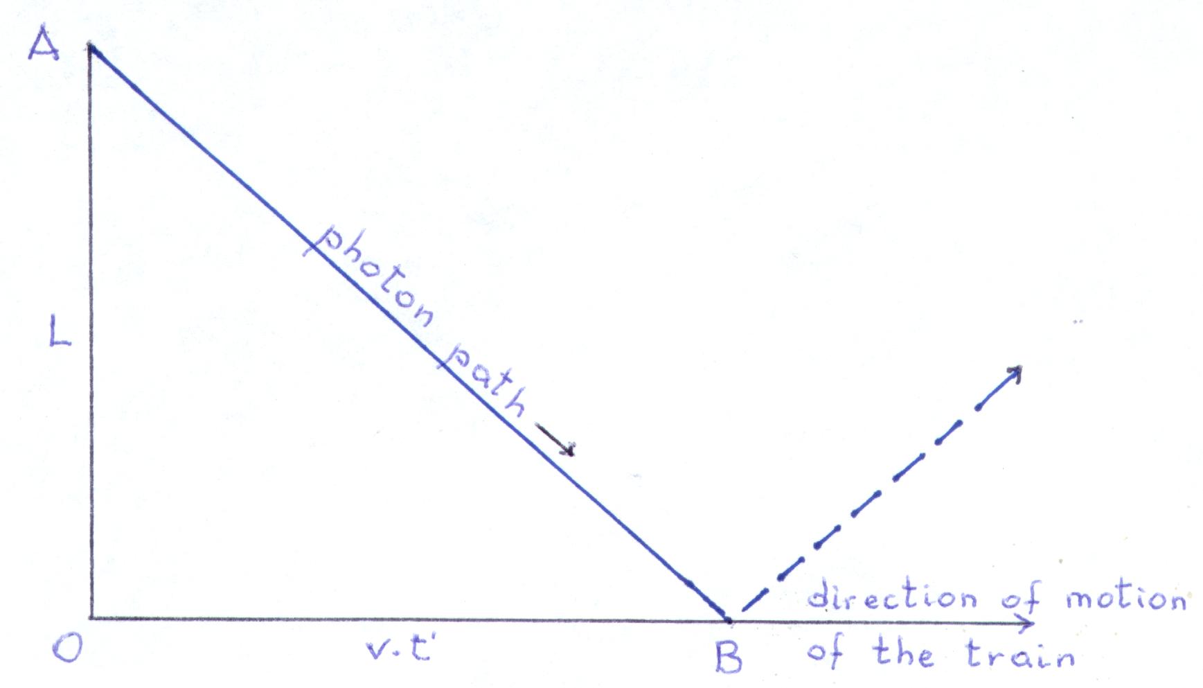
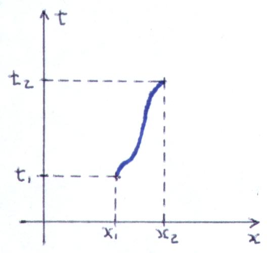
Avendo determinato che la velocità della luce è sempre la stessa in ogni direzione e in qualunque sistema di riferimento, a riposo rispetto alla terra oppure no, ora andiamo a considerare il fatto che il concetto di tempo dipende dalla velocità dell'osservatore. Esso diventerà più chiaro considerando la seguente situazione ipotetica: un tuo amico si trova in un treno che viaggia con velocità v e, mentre il treno corre veloce, egli gioca con una palla di gomma facendola rimbalzare sul pavimento del treno. La palla scende, rimbalza e ritorna alla sua mano. Si può calcolare facilmente sia il tempo che la palla impiega per raggiungere il pavimento, che quello che impiega per ritornare nella mano del lanciatore. Se la distanza tra la mano dell'amico e il pavimento è L e la palla si muove con velocità w, allora il tempo necessario per raggiungere il pavimento o tornare indietro è t = L / w. Questa è una semplice conseguenza del fatto che L = w · t, la quale deriva dalla definizione di velocità. Questa è una situazione molto semplice. Consideriamone ora una ipotetica e maggiormente interessante.

Supponi che il tuo amico non stia giocando con una palla di gomma, ma con... fotoni, cioè con raggi di luce! Ipoteticamente egli getta un fotone a terra dove ha posto uno specchio. Il fotone viene riflesso e ritorna al punto di partenza. Quanto impiega il fotone a raggiungere lo specchio sul pavimento o a tornare indietro? L'equazione è la stessa della palla di gomma. Tutto ciò che devi cambiare è la velocità. Devi mettere la velocità della luce c al posto della velocità w della palla di gomma. Quindi il tempo è t = L / c. Anche fino a questo punto tutto è semplice.

Considera adesso la stessa situazione, ma vista da fuori. Supponi di essere presso un passaggio a livello e di vedere il tuo amico che gioca con il fotone. (Come ho già detto, questa è una situazione ipotetica. Il fatto che tu non possa vedere il fotone che si muove e viene riflesso dallo specchio è irrilevante, come è irrilevante il fatto che non puoi udire il ticchettio dell'orologio del tuo amico in auto). Supponi di voler calcolare quanto tempo impiega il fotone a raggiungere lo specchio sul pavimento o a tornare indietro. In questo caso il calcolo è un po' più complicato perché mentre il fotone scende oppure sale il treno si sposta orizzontalmente con velocità v. Dal tuo punto di vista il cammino che il fotone percorre per raggiungere lo specchio è più lungo di quello che vede il tuo amico nel suo sistema di riferimento. Visto da te il fotone viaggia lungo una traiettoria simile a quella visualizzata nel grafico riportato qui sotto, il quale mostra schematicamente le caratteristiche essenziali del problema.

Quanto è lungo il cammino da A a B? Il tratto verticale OA è uguale a L. Se chiamiamo t' il tempo necessario al fotone per raggiungere il pavimento secondo il tuo punto di vista e se il treno viaggia con velocità v, allora il tratto orizzontale è OB = v · t'. Poiché il treno è in movimento e la velocità della luce non cambia, dal tuo punto di vista è richiesto un tempo maggiore perché il fotone raggiunga lo specchio sul pavimento.

Calcoliamo la relazione che esiste tra i due tempi, quello del tuo amico sul treno e il tuo. Lo possiamo ottenere facilmente per mezzo del teorema di Pitagora, il quale afferma che, dato un triangolo AOB, rettangolo in O, come quello mostrato nella figura, il quadrato della lunghezza dell'ipotenusa AB è uguale alla somma dei quadrati dei due cateti OA e OB, cioè AB² = OA² + OB². In altre parole, AB = √( OA² + OB² ).

Ora, se applichiamo il teorema al nostro caso, essendo OA = L e OB = v · t', otteniamo per la distanza tra A e B la seguente espressione: AB = √[ L² + ( v · t' )² ]. Questo è il cammino espresso in termini della velocità del treno che il fotone deve compiere per raggiungere il suolo. In termini della velocità della luce lo stesso intervallo ha la seguente forma: AB = c · t'. Uguagliando i quadrati dei due termini esprimenti AB, √[ L² + ( v · t' )² ] e c · t', e manipolando un poco l'equazione che ne deriva, otteniamo l'equazione che esprime t' in termini di L. Il risultato è:

t' = L / √( c² – v² ).

Compiamo ora un ulteriore sforzo. Sostituiamo L con c · t, cioè esprimiamo la lunghezza L in funzione del tempo dell'amico e arrangiamo di nuovo la formula. Il glorioso risultato finale è:

t' = t / √( 1 – v² / c² ).

Sottolineo il fatto che questa formula è stata ottenuta considerando la semplice lunghezza L per quanto riguarda l'amico, ma prendendo in considerazione nel tuo caso il percorso obliquo AB che trae origine dal moto del treno. Per questa ragione, come ho già menzionato, nel tuo sistema di riferimento il tempo richiesto dal fotone per raggiungere il pavimento è più lungo di quello che si sperimenta nel riferimento dell'amico. Di quanto? Come puoi vedere dalla formula, dipende dal rapporto v / c. Quando il treno è fermo, v / c = 0 e i due tempi coincidono. Come il treno parte succede quanto segue:

v / c > 0,

1 – v² / c² < 1,

1 / √( 1 – v² / c² ) > 1 e t' > t.

Se la velocità del treno dovesse avvicinarsi a quella della luce, allora

v / c → 1,

1 – v² / c² → 0,

1 / √( 1 – v² / c² ) → ∞ e t' >> t.

Osserva che in questo esperimento concettuale dal punto di vista del tuo amico non è coinvolto alcuno spazio nella direzione del moto. Questo è il motivo per cui il calcolo è così semplice. Forse avrai anche notato che, ogni volta che menziono intervalli di spazio o di tempo, specifico anche il sistema di riferimento. Questo è dovuto al fatto che gli intervalli di tempo e di spazio nella direzione del moto dipendono dal sistema di riferimento.

Ora uno si potrebbe chiedere perché io non abbia continuato a lavorare con la palla di gomma anziché introdurre il fotone, essendo che l'equazione che stabilisce la relazione tra il tempo e la distanza è la stessa. La ragione è che, mentre la velocità della luce è indipendente dal sistema di riferimento (il risultato fondamentale ottenuto dall'esperimento di Michelson e Morley), ciò non vale nel caso della palla di gomma.

Pagina principale

The time dilation

Having determined that the speed of light is always the same in any direction and from any point of view, whether one is at rest with respect to the earth or not, we're going to see now that the concept of time depends on the velocity of the observer. This concept will become more clear by considering a hypothetical situation. Suppose that your friend is on a train that is traveling with velocity v. While the train runs fast, he plays with a rubber ball, bouncing it on the train floor. The ball goes down and then bounces back to his hand. One can easily calculate the time it takes the ball to reach the floor and the time it takes to get back to the hand of the thrower. If the distance between your friend's hand and the floor is L and the ball travels with velocity w, than the time it takes to reach the floor or get back is t = L / w. This is a simple consequence of the fact that L = w ·t, which derives from the definition of velocity. This situation is very simple. Let us now consider a hypothetical, more interesting situation.

Suppose that your friend isn't playing with a rubber ball, but with... photons, that is, light! Hypothetically, he throws a photon to the floor where he put a mirror. The photon gets reflected and returns back to where it started. How long does it take for the photon to reach the floor, or to get back? The equation is the same as that of the rubber ball. All you need to change is the velocity, and put the speed of light c in place of the speed w of the rubber ball. Then the time is t = L / c. Also up to this point everything is very simple.

Consider now the situation as it's seen from another point of view. Suppose that you're near a train crossing, and see your friend playing with the photon. (As I said, this is a hypothetical situation. The fact that you cannot see the photon traveling and being reflected by the mirror is irrelevant, as was irrelevant the fact that you could not hear the ticks of your friend's clock in the car.) Suppose you want to calculate how long it takes for the photon to reach the mirror on the floor, or to get back (the duration is the same). The calculation is a little more difficult here, because, as the photon goes down, or up, the train moves horizontally with velocity v. From your point of view, the path the photon makes to reach the mirror is longer than the one seen from your friend's system of reference. As seen from you, the photon travels along a trajectory like the one shown on the graph below, which schematically shows the essential features of the problem.

How long is the path from A to B? The vertical path OA is still equal to L. If we call t' the time needed for the photon to reach the floor from your point of view and if the train travels with velocity v, then the horizontal path is OB = v · t'. Since the train is moving and the speed of light is the same in both frames, from your point of view it takes a longer interval of time for the photon to reach the mirror on the floor.

Let us calculate the relationship that exists between the two times, the one that applies to your friend on the train and the one relative to you. We can easily get it by means of Pythagoras' theorem, which says that, given a triangle AOB, squared in O, like the one shown on the figure, the square of the length of the hypotenuse AB is equal to the sum of the squares of the sides OA and OB, that is, AB² = OA² + OB². In other words, AB = √( OA² + OB² ).

Now, if we apply the theorem to our problem, since OA = L and OB = v · t', we obtain for the distance from A to B the following expression: AB = √[ L² + ( v · t' )² ]. This is the path expressed in terms of the velocity of the train that the photon has to make in order to reach the floor. In terms of the speed of light, the same interval has the following form: AB = c · t'. By equating the squares of the two terms that express AB, √[ L² + ( v · t' )² ] and c · t', and by manipulating the resulting equation a little bit, we obtain the relation that expresses t' in terms of L. The result is:

t' = L / √( c² – v² ).

Let us make now one last effort. We substitute L with c · t, that is, we express the length L in terms of your friend's time, and rearrange the formula again a little bit. The final, glorious result is:

t' = t / √( 1 – v² / c² ).

I stress that this formula has been obtained by taking into account the simple length L for what concerns your friend, but considering in your case the oblique path AB that arise from the motion of the train. For this reason, as I mentioned before, in your frame of reference the time the photon needs to get to the floor is longer than the one experienced in your friend's frame. By how much? As you can see from the formula, it depends on the ratio v / c. When the train is at rest, v / c = 0, and the two times coincide. On the other hand, as the train moves,

v / c > 0,

1 – v² / c² < 1,

1 / √( 1 – v² / c² ) > 1, and t' > t.

Should the velocity of the train get close to the speed of light, then

v / c →1,

1 – v² / c² → 0,

1 / √( 1 – v² / c² ) → ∞, and t' >> t.

Observe that in this conceptual experiment from the point of view of your friend there is no space involved in the direction of motion. This is the reason why the calculation is so simple. Perhaps you also noticed that almost every time that I mention a space or time interval I also specify the frame of reference. This is because the time intervals and the space intervals in the direction of motion are frame dependent.

One might ask why I didn't continue to work with the rubber ball and its speed instead of introducing the photon, as the equation that relates time and distance is the same in both cases. The reason is that, while the speed of light is frame independent (the fundamental result obtained by the Michelson and Morley experiment), this is not true in the case of the velocity of the rubber ball.

Home

La contrazione dello spazio

Consideriamo una situazione un po' più complicata. Ora l'amico appende uno specchio sulla parete di fronte e ricomincia a giocare con i fotoni. Essi vanno dalla lampada dell'amico allo specchio e tornano indietro. Nello stesso tempo il treno continua a muoversi nella direzione puntata dalla lampada. Se la distanza tra la lampada e lo specchio è L, il tempo che un fotone impiega a percorrere tale distanza è t_f = L / c, e quello che impiega per tornare indietro è ugualmente t_b = L / c. Il tempo totale tra partenza e ritorno alla lampada è

(3.1): t = t_f + t_b = 2 · L / c.

Dal tuo punto di vista, però, nel mentre che il fotone viaggia dalla lampada allo specchio anche il treno si muove nella stessa direzione. Perciò, quando il fotone giunge al punto dove stava lo specchio inizialmente, esso si è spostato un poco in avanti e il fotone deve continuare a muoversi. Per quanto tempo? Se t_f' è il tempo necessario per andare dalla lampada allo specchio, essendo che in quel tempo lo specchio avanza di v · t_f', la distanza totale che il fotone deve percorrere è L_f' = L' + v · t_f'. Poniamo L' invece di L perché è da aspettarsi che il suo valore cambi. Espressa mediante la velocità della luce, la distanza che il fotone deve percorrere è c · t_f'. Uguagliando le due espressioni della distanza, ( L' + v · t_f' = c · t_f' ) e risolvendo rispetto a t_f', otteniamo

t_f' = L' / ( c – v ) = ( L' / c ) / ( 1 – v / c ).

Come viene riflesso, il fotone prende il cammino del ritorno e percorre la distanza c · t_b'. D'altra parte, per il fatto che il treno continua a muoversi, la distanza che il fotone deve percorrere è L' – v · t_b'. Come nel caso precedente, uguagliamo queste due distanze e risolviamo l'equazione rispetto a t_b'. Il risultato è

t_b' = ( L' / c ) / ( 1 + v / c ).

Un semplice calcolo mostra che il tempo totale necessario al fotone per andare e ritornare è

(3.2): t' = t_f' + t_b' = ( 2 · L' / c ) / ( 1 – v² / c² ) .

Ora dovremmo confrontare le formule (3.1) e (3.2), ma esse non usano né lo stesso tempo né lo stesso spazio. Come facciamo? Chiamiamo in aiuto la relazione tra il tempo dell'amico e il tuo (vedi La dilatazione del tempo): t' = t / √( 1 – v² / c² ). Introducendo l'espressione di t' nell'equazione (3.2) e semplificando otteniamo:

(3.3): t = ( 2 · L' / c ) / √( 1 – v² / c² ).

Ora possiamo confrontare le equazioni (3.1) e (3.3). Infine otteniamo:

L' = L · √( 1 – v² / c² ).

Da questa formula vediamo che, come la velocità del treno aumenta, il fattore con la radice quadrata decresce. Perciò, visto da te, le distanze nella direzione del moto del treno sono contratte, e se la velocità del treno ipotetico dovesse raggiungere la velocità della luce, tanto √( 1 – v² / c² ) che L' tenderebbero a zero.

Si può comprendere la contrazione dello spazio in termini meno rigorosi nella seguente maniera. Come aumenta la velocità del treno, dal tuo punto di vista il fotone deve percorrere distanze sempre maggiori per raggiungere lo specchio e, se non fosse per la contrazione dello spazio, il tempo richiesto perché il fotone compia il viaggio di andata e ritorno sarebbe troppo lungo. Infatti, se mettiamo in (3.3) L al posto di L', per v > 0 l'espressione risultante per il tempo t non coincide con quella ottenuta dalla (3.1). Perciò, per ottenere il tempo corretto nel tuo riferimento gli intervalli spaziali nella direzione del moto del treno devono essere ridotti.

Pagina principale

The space contraction

Let us consider a situation a little more complicated. Now your friend hangs the mirror to the wall in front of him and starts playing again with photons. They go from your friend's lamp to the mirror and back. At the same time the train keeps moving in the direction pointed by the lamp. If L is the distance between the lamp and the mirror, the time a photon takes to travel that distance is t_f = L / c, and the one it takes to get back is t_b = L / c. The total time between departure and arrival back to the lamp is

(3.1): t = t_f + t_b = 2 · L / c.

From your point of view, however, as the photon travels from the lamp to the mirror, the train also moves in the same direction. As the photon arrives at the point where initially the mirror was, the mirror has moved ahead a little bit, and the photon keeps on moving. For how long? If t_f' is the time necessary for going from the lamp to the mirror, since during that time the mirror moves ahead by v · t_f', the total distance the photon has to travel is L_f' = L' + v · t_f'. We put L' instead of L because we expect it to be different from L. In terms of the speed of light, the distance the photon has to travel is c · t_f'. By equating the two expressions for the distance (  L' + v · t_f' = c · t_f' ) and by solving with respect to t_f', we get

t_f' = L' / ( c – v ) = ( L' / c ) / ( 1 – v / c ).

Being reflected, the photon starts going back and travels the distance c · t_b'. On the other hand, as the train keeps moving, the distance the photon has to travel is L' – v · t_b'. Like before, we equate these two distances and solve with respect to t_b'. The result is

t_b' = ( L' / c ) / ( 1 + v / c ).

A simple calculation shows that the total time the photon needs for going forward and back is

(3.2): t' = t_f' + t_b' = ( 2 · L' / c ) / ( 1 – v² / c² ).

Now we should compare the formulas (3.1) and (3.2), but they have nothing in common. How do we do it? We call to the rescue the relationship between your friend's time and yours (see The time dilation): t' = t / √( 1 – v² / c² ). Substitution of this expression for t' into equation (3.2) and simplification gives:

(3.3): t = ( 2 · L' / c ) / √( 1 – v² / c² ).

Now we can compare equations (3.1) and (3.3). We finally get:

L' = L · √( 1 – v² / c² ).

From this formula we see that, as the train velocity increases the root factor decreases. Hence, seen from you the distances in the direction of motion of the train are contracted and, as the velocity of the hypothetical train approaches the speed of light, both √( 1 – v² / c² ) and L' tend to zero.

One can understand the space contraction in less rigorous terms also in this way. As the velocity of the train increases, from your point of view the photon has to travel longer and longer distances to catch the mirror and, were it not for the space contraction, the time required for the photon to go forward and back would be too long. In fact, if we put in (3.3) L instead of L', when v > 0 the resulting expression for t does not match the one obtained in (3.1). So, in order to get the correct time, in your reference the space intervals in the direction of motion must be reduced.

Home

Contemporaneità un relatività

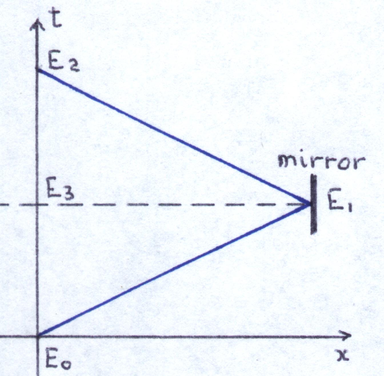
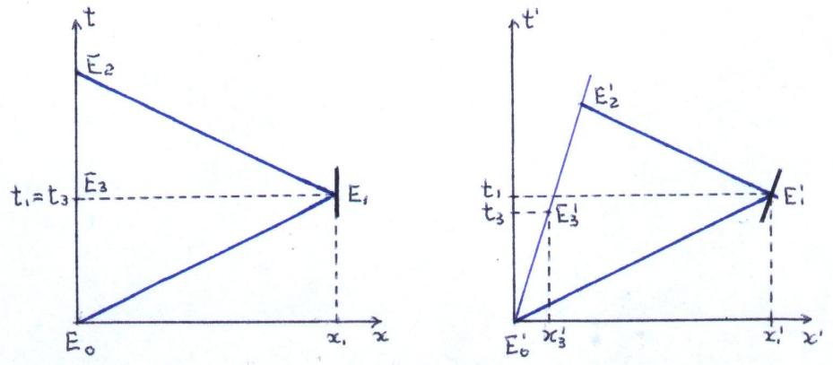
Quello di contemporaneità è un concetto ovvio; gli eventi simultanei sono caratterizzati dalla stessa coordinata temporale. Vediamo cosa succede di due eventi simultanei quando si cambia sistema di riferimento. Prendiamo in considerazione la situazione descritta in La contrazione dello spazio, dove l'amico sta viaggiando in treno (egli ama viaggiare) e tu stai presso un passaggio a livello (a te piace guardare i treni che passano). Riguardo al suo sistema di riferimento, se fissiamo l'origine del tempo nel momento in cui il fotone lascia la lampada, tale evento è caratterizzato da t₀ = 0. Al tempo t₁ = L / c il fotone raggiunge lo specchio che sta di fronte all'amico. Al tempo t₂ = 2 · L / c il fotone è di ritorno e colpisce la lampada. Sia E₃ l'evento sulla lampada contemporaneo a E₁. Nel sistema di riferimento dell'amico esso è caratterizzato da t₃ = t₁ = L / c.

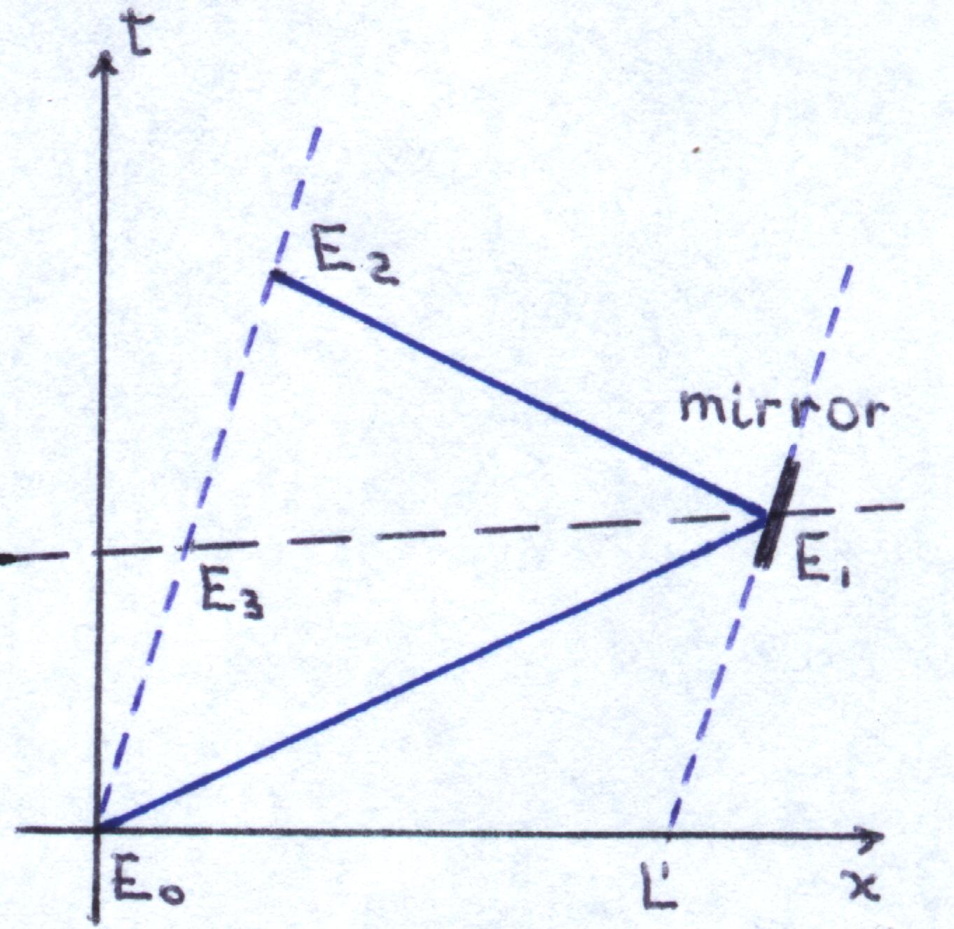
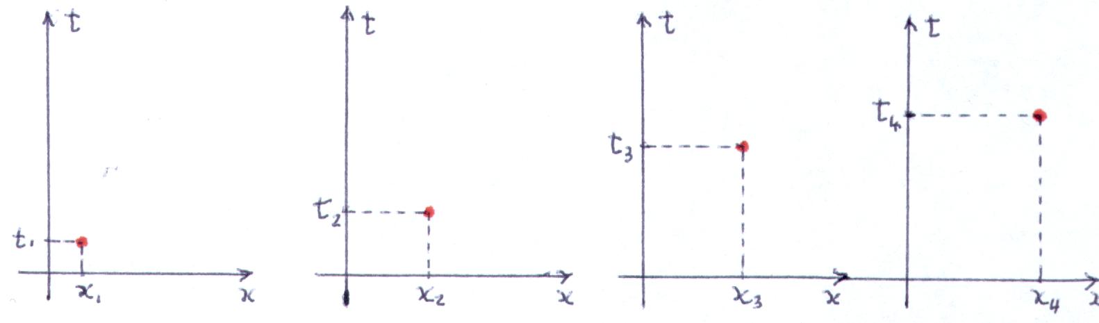
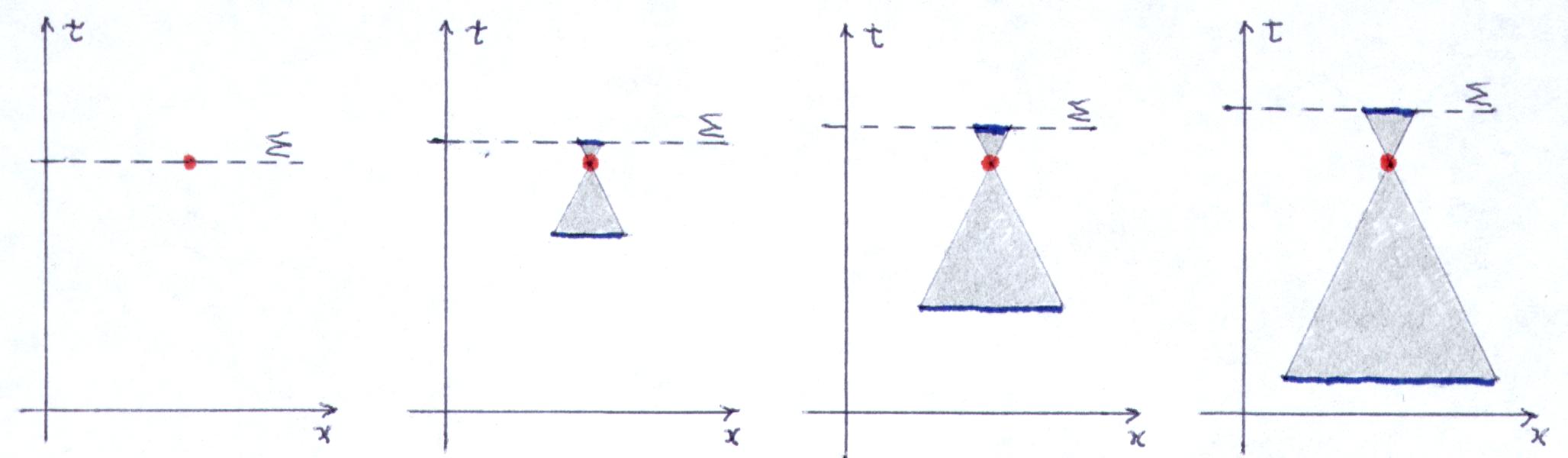
Cambiamo adesso sistema di riferimento. Ci portiamo sul tuo e determiniamo i tempi che corrispondono a E₁ e E₃. Se prendiamo come origine degli assi il momento in cui il fotone lascia la lampada, allora l'evento associato al fotone che raggiunge lo specchio è caratterizzato da

(4.1): t₁' = t_f' = ( L' / c ) / ( 1 – v / c ),

secondo la spiegazione data in La contrazione dello spazio. Come facciamo a ricavare il tempo che corrisponde a E₃? Poiché questo evento si trova in mezzo tra E₀ ed E₂, ed essendo t₀ = 0, non dobbiamo far altro che calcolare t₂' e dividerlo per due. Ora t₂' è la somma dei tempi necessari al fotone per andare e tornare, cioè, t₂' = t_f' + t_b'. Quindi, tenendo conto dell'espressione t_b' = L' / ( c – v ) ricavata in La contrazione dello spazio, otteniamo

(4.2): t₃' = ( t_f' + t_b' ) / 2 = ( L' / c ) / ( 1 – v² / c² ).

Confrontando (4.1) e (4.2) si può vedere che per ogni v maggiore di zero e minore di c (0 < v < c, o equivalentemente, 0 < v / c < 1), il fattore 1 / ( 1 – v² / c² ) è minore di 1 / ( 1 – v / c ). Lo si può verificare facilmente osservando che

1 / ( 1 – v² / c² ) = [ 1 / ( 1 – v / c ) + 1 / ( 1 + v / c ) ] / 2

< 1 / ( 1 – v / c ) = [ 1 / ( 1 – v / c ) + 1 / ( 1 – v / c ) ] / 2.

L'unica differenza tra le due espressioni è quella sottolineata. Poiché

1 + v / c > 1 – v / c,

di conseguenza

1 / ( 1 + v / c ) < 1 / ( 1 – v / c ),

e

1 / ( 1 – v² / c² ) < 1 / ( 1 – v / c ).

Dal confronto di (4.1) e (4.2) si comprende che nel tuo riferimento E₃ è sempre in ritardo rispetto a E₁. Ciò che è simultaneo nel riferimento dell'amico non è contemporaneo nel tuo. Il grafico che segue mostra le posizioni dei vari eventi secondo il tuo punto di vista

Nel tuo sistema di riferimento gli eventi che sono contemporanei in treno appaiono disporsi su una linea obliqua. Dal grafico vediamo un'altra ragione per cui gli intervalli spaziali sono contratti. Essa risiede nel fatto che, sebbene la lunghezza del segmento E₁ – E₃ sia aumentata a motivo del moto, nel tuo riferimento esso è ruotato verso il futuro. Nota anche che, essendo la misura eseguita in un tempo specifico, la lunghezza che appare nel tuo sistema di riferimento non è la proiezione di E₁ - E₃ ortogonale all'asse x (cioè la posizione che lo specchio raggiunge più tardi), ma piuttosto è la proiezione lungo la linea di moto. Più il segmento E₁ - E₃ ruota e più corta è la parte dell'asse spaziale che è individuato dalle linee di moto. Se il treno dovesse muoversi (ipoteticamente) alla velocità della luce, allora il segmento L si disporrebbe parallelamente al raggio di luce e la lunghezza della sua proiezione sull'asse spaziale si ridurrebbe a zero. Tuttavia le particelle con massa diversa da zero non possono mai raggiungere la velocità della luce.

Pagina principale

Contemporaneity in relativity

Contemporaneity is an obvious concept. Simultaneous events are characterized by the same value of the time coordinate. Let's see what happens of two events, simultaneous in one coordinate system, when we pass to another system of reference. We take into account the situation described in The Space Contraction, where your friend is traveling on a train (he likes traveling), and you're standing near a train crossing (you like watching trains passing by). Regarding his frame of reference, if we fix the time origin at the moment when a photon leaves the lamp your friend is holding, this event is characterized by t₀ = 0. At t₁ = L / c the photon reaches the mirror in front of him. At t₂ = 2 · L / c the photon is back and hits the lamp. Let's call E₃ the event on the lamp contemporaneous to E₁. In your friend's reference it's characterized by t₃ = t₁ = L / c.

We now change system of reference. We move in yours and determine the times that correspond to E₁ and E₃. If we take as time origin the moment in which the photon leaves the lamp, then the event when the photon reaches the mirror is characterized by

(4.1): t₁' = t_f' = ( L' / c ) / ( 1 – v / c ),

according to the explanation given in The Space Contraction. How do we get the time that corresponds to E₃? Since this event is in the middle between E₀ and E₂, and t₀ = 0, all we have to do is calculate t₂' and divide it by two. Now t₂' is the sum of the times needed to go forward and back, that is t₂' = t_f' + t_b'. Hence, by taking into account the expression t_b' = L' / ( c – v ) we got in The Space Contraction, we obtain

(4.2): t₃' = ( t_f' + t_b' ) / 2 = ( L' / c ) / ( 1 – v² / c² ).

By comparing (4.1) and (4.2), you can see that for any v larger than zero and smaller than c (0 < v < c, or equivalently, 0 < v / c < 1), the factor 1 / ( 1 – v² / c² ) is smaller than 1 / ( 1 – v / c ). The verification is simple by noting that

1 / ( 1 – v² / c² ) = [ 1 / ( 1 – v / c ) + 1 / ( 1 + v / c ) ] / 2

< 1 / ( 1 – v / c ) = [ 1 / ( 1 – v / c ) + 1 / ( 1 – v / c ) ] / 2.

Only the underlined parts are different. Since

1 + v / c > 1 – v / c,

consequently

1 / ( 1 – v² / c² ) < 1 / ( 1 – v / c ).

and

1 / ( 1 – v² / c² ) < 1 / ( 1 – v / c ).

By comparing (4.1) and (4.2), this result shows that in your reference E₃ is always retarded with respect to E₁. What is simultaneous in your friend's reference is not contemporaneous in yours. The following graph shows the positions of the various events as they appear in your reference.

In your system of reference the events that in the train are contemporaneous appear lying on an oblique line. From the graph we also see another reason why space intervals get contracted. It lies in the fact that, although the length of the segment E₁ – E₃ is increased because of the motion, in your frame it's rotated toward the future. Note also that, since the measure is made at a specific time, the length that appears in your system of reference isn't the projection of E₁ – E₃ orthogonal to the x axis (that position is reached later), but rather its projection along the line of motion. The more the segment E₁ – E₃ rotates and the shorter is the part of the spatial axis that is crossed. Had the train to move (hypothetically) at the speed of light, the segment L would point along the light ray and the length of its projection on the spatial axis would reduce to zero. However, particles with non-zero mass can never reach the speed of light.

Home

Evidenze relativistiche

É tempo di introdurre alcuni esempi che mostrino che le dilatazioni dei tempi e le contrazioni degli spazi sono reali. Potrei dire che la loro veracità è convalidata quotidianamente nei laboratori di tutto il mondo, perché altrimenti gli esperimenti non funzionerebbero a dovere, ma credo che una tale asserzione non soddisferebbe la maggior parte dei lettori. Perciò menziono alcuni esempi che dimostrano la tesi. Il primo è una manifestazione sia di dilatazione del tempo che di contrazione dello spazio, a seconda del sistema di riferimento.

Poiché le modifiche degli intervalli di spazio e di tempo sono per lo più evidenti in circostanze straordinarie, quando la velocità coinvolta è dell'ordine di quella della luce, dobbiamo considerare situazioni molto singolari. Una tale occorrenza avviene quando i raggi cosmici colpiscono l'alta atmosfera. Questi sono costituiti da particelle con elevata energia cinetica, con velocità elevatissime, paragonabili come ordine di grandezza a quella della luce. Quando queste particelle originarie del cosmo raggiungono l'alta atmosfera, a circa 50.000 metri di altitudine, esse interagiscono con i gas tenui lì presenti. Di conseguenza, similmente a quanto accade negli acceleratori di particelle sulla terra, le collisioni danno origine a nuove particelle, alcune delle quali, come i muoni, hanno vite medie molto brevi. Se non fosse per la dilatazione del tempo e la contrazione dello spazio esse non potrebbero raggiungere la superficie della terra, ma decaderebbero subito dopo essere venute all'esistenza. Al contrario, esse sono parte dei raggi cosmici che giungono sulla terra, nonostante la loro durata di vita sia così breve (la vita media dei muoni è di circa 2 milionesimi di secondo) che anche procedendo ad una velocità prossima a quella della luce si disintegrerebbero dopo poche centinaia di metri.

Vediamo come la dilatazione del tempo e la contrazione dello spazio rende loro possibile raggiungere la terra. Dal nostro punto di vista la distanza che il muone deve percorrere, circa 50 chilometri, non è modificata per niente. Tuttavia, poiché la durata della vita nel loro sistema di riferimento è molto breve, dal nostro punto di vista questo brevissimo intervallo di tempo si allunga così tanto che una porzione considerevole di essi è in grado di raggiungere la terra senza disintegrarsi. La dilatazione del tempo rende loro possibile rimanere intatti per centinaia se non migliaia di volte più a lungo di quando non lo siano nel loro riferimento.

E riguardo alla contrazione dello spazio? Supponiamo di stare seduti sopra un muone che è appena venuto all'esistenza. Allora dal nostro punto di vista non c'è alcuna dilatazione del tempo e la particella esiste senza disintegrarsi per un brevissimo periodo di tempo e prima che riesca a percorrere alcune centinaia di metri è già disintegrata. Come può allora raggiungere la superficie della terra? Da quel punto di vista la terra si va avvicinando molto rapidamente, ad una velocità prossima a quella della luce. Ora il ruolo qui svolto è la contrazione dello spazio invece della dilatazione del tempo. Da quel punto di vista la distanza tra l'alta atmosfera e la superficie della terra è contratta e lo spazio che il muone deve percorrere è molto breve, così che esso è in grado di raggiungere la terra. Dal punto di vista della particella il tempo procede normalmente, ma la terra appare come se fosse quasi piatta.

Un'altra verifica della teoria è stata effettuata in passato mediante i satelliti artificiali. I satelliti non si muovono a velocità confrontabili con quella della luce, ma ciononostante essi costituiscono i mezzi più veloci disponibili su cui poter porre un orologio. Sono stati condotti degli esperimenti in cui si è posto un orologio molto preciso su un satellite, e il suo 'ticchettio' è stato confrontato con quello di un orologio identico sulla terra. L'orologio sul satellite è risultato più lento di quello sulla terra, come predetto dalla teoria della relatività.

Come ho già detto, quando due orologi si muovono l'uno rispetto all'altro, ogni orologio nel proprio riferimento è più veloce dell'altro. Allora ci si può chiedere: se l'orologio che si muove, rallenta e si ferma, perché dovrebbe indicare un tempo diverso da quello che è sempre rimasto fermo? Non dovrebbero i due tempi coincidere dopo che si sono aggiustate le loro velocità? No. Questo è un aspetto che porta a dire che se ci sono due gemelli ed uno di loro fa un viaggio su un'astronave, al suo ritorno riscontrerà che il fratello rimasto sulla terra è invecchiato più di lui. Come si spiega questo fatto? Riflettiamo su questo: cosa c'è di diverso tra il gemello rimasto sulla terra e quello che ha compiuto il viaggio? La risposta è: nel caso del gemello viaggiatore è coinvolta l'accelerazione. Dapprima egli è soggetto ad un'accelerazione che lo porta a raggiungere una velocità prossima a quella della luce, poi ad una decelerazione, ecc. Durante le accelerazioni e decelerazioni le cose si aggiustano così che alla fine del viaggio il gemello dell'astronave è più giovane del fratello che è rimasto sulla terra. Questo non significa che colui che viaggia viva più a lungo, ma semplicemente che dal suo punto di vista il tempo necessario per compiere l'intero viaggio è più breve di quanto che appare dal punto di vista della terra.

La dilatazione del tempo e la contrazione dello spazio sono due aspetti che si manifestano ogni volta che si passa da un sistema di riferimento ad un altro. Le lunghezze degli intervalli di tempo e di spazio dipendono da chi le misura, dal suo stato di moto. É interessante notare che spazio e tempo non sono le sole grandezze che si comportano in questa maniera. Vedremo più avanti che ci sono altre grandezze fisiche che pure ubbidiscono alla stessa legge. Ciò giocherà un ruolo importante nel comprendere la ragione per cui spazio e tempo si comportano in tale maniera. Ma prima è importante comprendere meglio come gli intervalli dello spazio-tempo si trasformano nel passare da un sistema di riferimento ad un altro. Perciò nel prossimo capitolo prenderemo in considerazione la trasformazione di Lorentz.

Pagina principale

Relativistic evidences

It's time to introduce some evidences showing that time dilations and space contractions are not fantasy, but real. I could say that the truthfulness of the theory is validated every day in the laboratories around the world because without it many experiments would not work, but I believe that such statement would not satisfy most of the readers. So I mention a few examples that prove the thesis. The first one shows a manifestation of both the time dilation and space contraction, depending on the system of reference.

Since the modifications of the space and time intervals are mostly evident under the extraordinary condition in which the speed involved is close to that of light, we must look at peculiar situations. One such occurrence happens when the cosmic rays hit the upper atmosphere. Cosmic rays are made up of very energetic particles. Their speeds are very high, comparable to the speed of light. When these particles that originate in the cosmos reach the upper atmosphere, at about 50,000 meters, they interact with the tenuous gases they find there. As a consequence, similarly to what happens in the particle accelerators on earth, the collisions give rise to new particles, some of which, like the muons, have very short mean lives. Were it not for the time dilation and space contraction, they'd never reach the surface of the earth, but decay shortly after being created. Instead, they're part of the cosmic rays that arrive on earth, although their life span is so short (the muon mean life is about 2 millionth of a second) that, even by proceeding at a speed close to that of light, they would disintegrate after a few hundred meters.

Let us see how time dilation and space contraction make it possible for them to reach the surface of the earth. From our point of view the distance the muons have to travel, about 50 kilometers, isn't modified at all. However, no matter the fact that their life span in their system of reference is very short, from our point of view that tiny interval of time is stretched so much that a considerable portion of them are able to travel down to earth without disintegrating. Time dilation makes them possible to live hundreds if not thousands of times longer than they actually do in their own frame.

What about space contraction? Suppose you're sitting on a muon that has just been created. Then from that point of view there's no time dilation and the particle lives for a very short time; before traveling a few hundred meters it disintegrates. How can it reach the surface of the earth? From that point of view the earth is approaching very fast, at a velocity close to that of light. Now the role played here is space contraction instead of time dilation. From that point of view, the distance from the upper atmosphere to the surface of the earth is contracted, the space the muon has to travel is very short, and that enables it to reach the surface. From the particle point of view time proceeds normally, but the earth appears as if it were almost flat.

Another verification of the theory has been made in the past by means of satellites. Satellites do not move at speeds comparable to that of light, nonetheless they constitute the fastest means available today on which to put a clock. Experiments have been made in which a very precise clock has been put on a satellite and its ticking has been compared with that of an identical clock on earth. The clock on the satellite ticked slower than the one on earth, as predicted by the theory of relativity.

As I said earlier, when two clocks are moving with respect to one another, from its point of view each clock runs faster than the other one. Then one might ask: if the moving clock slows down and comes to rest, why should it show a time different from the one that had always remained at rest? Should not the two times coincide after the velocities have been adjusted? No. This is the aspect that leads to say that if there is a couple of twins and one of them makes a long journey on a spaceship, on coming back to earth he'd find his twin brother aged more than himself. How can it be explained? Think about this: what is the difference between the twin that remains on earth and the one that makes the space travel? The answer is: in the case of the traveling twin, acceleration is involved. First he is subject to an acceleration that brings him close to the speed of light, then to a deceleration, and so on. During the accelerations and decelerations things get adjusted so that at the end of the trip the twin in the spaceship is younger than his brother that remained on earth. This does not mean that the one that travels is going to live longer, but simply that from his point of view the time needed to make the journey is shorter than what appears from the earth point of view.

Time dilation and space contraction are two aspects that get manifested every time one passes from one system of reference to another. Space and time lengths depend on who measures them, on his state of motion. It is interesting to note that space and time are not the only quantities that behave like this. We shall see later on that there are other physical quantities that get modified by motion. This aspect will play a significant role in understanding the reason why space and time behave as they do. But first it's important to understand better how the coordinates of space-time intervals transform from one system of reference to another. So, in the next chapter we'll consider this aspect.

Home

La trasformazione di Lorentz

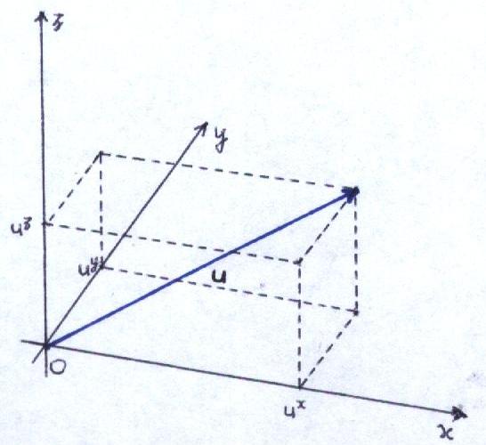
Prima di esaminare la trasformazione di Lorentz, consideriamo brevemente il concetto di quadrivettore, o 4-vettore. Per 4-vettore si intende una freccia nello spazio-tempo tetradimensionale. Dato un sistema di quattro assi ortogonali con origine sulla parte posteriore della freccia, un 4-vettore può essere rappresentato dalle proiezioni, o componenti, della sua punta sugli assi ortogonali del sistema di coordinate (nota: per semplicità mi limito a considerare il caso in cui gli assi siano ortogonali). Il grafico sottostante mostra un vettore e le sue componenti nel caso più semplice di uno spazio a tre dimensioni.

Per indicare un vettore di tipo spazio useremo la notazione abbreviata u, e u^x, u^y, u^z per le sue componenti lungo gli assi x, y, z. A volte è utile porre le componenti tra parentesi, come in (u^x, u^y, u^z). Un'altra utile notazione è uⁱ, dove la lettera latina i (oppure j, k, ecc.) posta come apice può assumere uno qualsiasi dei valori 1, 2 e 3, i quali stanno a rappresentare x, y e z. In riferimento ai vettori di tipo spazio, le notazioni u, uⁱ, (u¹, u², u³) e (u^x, u^y, u^z) si equivalgono. Per quanto riguardo i 4-vettori dello spazio-tempo è consuetudine usare la notazione u^μ, dove la lettera greca μ (pronuncia 'mu') può assumere qualsiasi valore intero compreso tra 0 e 3, con la convenzione che u⁰ sta ad indicare la componente di tipo tempo. Perciò u^μ, (u⁰, u), (u⁰, u¹, u², u³) e (u^t, u^x, u^y, u^z) sono notazioni differenti che rappresentano lo stesso 4-vettore. A volte gli indici possono apparire nella parte inferiore, come in u_μ. Non ne spiego qui il motivo: accettali come sono.

Consideriamo la trasformazione di Lorentz, la legge che specifica il modo in cui gli intervalli spaziali e temporali si trasformano nel passare da un sistema di riferimento ad un altro. Lorentz introdusse la sua legge di trasformazione in modo che fosse in accordo con le leggi dell'elettromagnetismo. Infatti, prima di questa legge erano sorte difficoltà con la teoria dell'elettromagnetismo per il fatto che le sue leggi apparivano dipendere dal sistema di riferimento, il che spinse Michelson e Morley a compiere il loro famoso esperimento. In quel tempo si pensava che la legge scoperta da Lorentz si applicasse solo all'elettromagnetismo. Solo con la pubblicazione della teoria della relatività da parte di Einstein apparve chiaro che la legge di Lorentz andava applicata a tutti i fenomeni fisici (tutto è relativo). Vedremo meglio questo aspetto in un prossimo capitolo, quando sarà trattata la teoria della relatività. Per il momento andiamo ad esaminare la legge a cui sono soggette le componenti spaziali e temporali dei quadrivettori quando si cambia sistema di riferimento. Nell'ottenerla useremo le seguenti espressioni ricavate in La contrazione dello spazio:

(6.1): t_f' = ( L' / c ) / ( 1 – v / c ) = ( L / c ) · √( 1 – v² / c² ) / ( 1 – v / c ),

(6.2): t_b' = ( L' / c ) / ( 1 + v / c ) = ( L / c ) · √( 1 – v² / c² ) / ( 1 + v / c ),

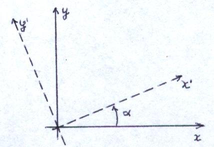
Per esprimere le componenti spaziali e temporali dei 4-vettori del sistema a riposo in termini di quelle dell'altro (vedi grafici), consideriamo le coordinate dell'evento E₁': t₁' e x₁'. Nel riferimento del treno il vettore E₁ – E₀ è la somma del vettore puramente temporale, E₃ – E₀, e di quello puramente spaziale, E₁ – E₃. Le coordinate del primo vettore sono E₃ – E₀ = (t₃, 0) = (t₁, 0) e quelle del secondo vettore sono E₁ – E₃ = (t₁ – t₃, x₁) = (0, x₁). I vettori corrispondenti nel sistema a riposo sono E₃' – E₀' = (t₃', x₃') e E₁' – E₃' = (t₁' – t₃',  x₁' – x₃').

Proponiamoci ora di determinare t₃' in termini di t₃. Ricordando che t₃' = ( t_f' + t_b' ) / 2 e usando (6.1) e (6.2) otteniamo:

(6.3): t₃' = ( L / c ) / √( 1 – v² / c² ).

Di conseguenza:

(6.4): x₃' = v · t₃' = ( v · L / c ) / √( 1 – v² / c² ).

Nel riferimento sul treno E₃ – E₀ è puramente temporale. Perciò in (6.3) e (6.4) poniamo t₁ (= t₃) al posto di L / c:

t₃' = t₁ / √( 1 – v² / c² ),

x₃' = ( v · t₁ ) / √( 1 – v² / c² ).

Ciò che abbiamo ottenuto in (6.3) and (6.4) ci aiuta a ricavare anche le componenti temporale e spaziale di E₁' – E₃'. Dopo qualche calcolo giungiamo a:

t₁' – t₃' = t_f' – t₃' = ( v · L / c² ) / √( 1 – v² / c² ),

x₁' – x₃' = c · t_f' – v · t₃' = L / √( 1 – v² / c² ).

Nel riferimento del treno, l'intervallo L è di tipo spazio. Perciò sostituiamo L con x₁:

(6.5): t₁' – t₃' = ( v · x₁ / c² ) / √( 1 – v² / c² ),

(6.6): x₁' – x₃' = x₁ / √( 1 – v² / c² ).

Infine, sommando (6.3) e (6.5) otteniamo:

t₁' = ( t₁ + x₁ · v / c² ) / √( 1 – v² / c² ),

mentre la somma di (6.4) e (6.6) produce:

x₁' = ( x₁ + v · t₁ ) / √( 1 – v² / c² ).

Questa è la trasformazione di Lorentz delle due coordinate t₁ e x₁. Nella letteratura di solito si usa il simbolo γ (pronuncia 'gamma') al posto di 1 / √( 1 – v² / c² ). Operando la sostituzione, togliendo l'indice 1 da t₁ e x₁ e ricordando che le coordinate y e z non sono influenzate dal moto, la trasformazione di Lorentz completa per questo caso particolare acquista la seguente forma:

(6.7): t' = ( t + x · v / c² ) · γ;, x' = ( x + v · t ) · γ, y' = y, z' = z.

Prima dello sviluppo delle teorie dell'elettromagnetismo e della relatività si riteneva che il tempo non fosse influenzato dal moto dell'osservatore: (t' = t). La correzione operata da γ su x' è molto piccola per velocità ordinarie. É un effetto puramente relativistico che si manifesta in particolar modo ad alte velocità. Senza il fattore γ e con t' = t la formula è conosciuta come trasformazione di Galilei, e va applicata quando gli effetti relativistici sono trascurabili. Si dovrebbe osservare che il fattore γ influenza sia la coordinata spaziale nella direzione del moto che quella temporale, il che significa che il moto le dilata entrambe. Riguardo allo spazio, ciò che viene contratta non è la proiezione della distanza L presa ortogonalmente all'asse x, ma la sua proiezione lungo la direzione di moto del treno nel piano (t', x').

A voler essere rigorosi la trasformazione (6.7) non è la più generale, ma quella a cui di solito ci si riferisce quando si parla di trasformazione di Lorentz, perché è quella parte della trasformazione più generale che differisce dalla corrispondente trasformazione di Galilei. Una generica trasformazione di Lorentz include le rotazioni, ossia, la più generale trasformazione di Lorentz è una combinazione di molteplici rotazioni e di una trasformazione tipo quella che abbiamo ricavato. Per completezza mostro senza dimostrazione un esempio di rotazione. Dato un angolo di rotazione α nel piano (x, y), ecco come vengono trasformati gli assi x e y:

x' = x · cos(α) + y · sin(α), y' = – x · sin(α) + y · cos(α).

Pagina principale

The Lorentz transformation

Before considering the Lorentz transformation, let's briefly examine the concept of 4-vector. By 4-vector we mean an arrow in four-dimensional space-time. Given a set of four orthogonal axes with origin on the back of the arrow, the 4-vector can be represented by its projections, or components, on the orthogonal axes of the system of coordinates (note: the axes do not necessarily need to be orthogonal, but for simplicity we limit ourselves to this particular case). The graph below shows a vector and its components in the simpler case of a three dimensional space.

Ordinarily, the notation u is used for short to indicate a space-like vector, and u^x, u^y, u^z for its components along the x, y, z axes. Sometimes it's convenient to put the components within brackets, like (u^x, u^y, u^z). Another useful notation for a vector is uⁱ, where the upper Latin letter i (or j, k, etc.) may take any of the values 1, 2 and 3, and such indices stand for x, y and z. In the case of space-like vectors, the notations u, uⁱ, (u¹, u², u³) and (u^x, u^y, u^z) are equivalent. In dealing with 4-vectors related to space-time, it's customary to use the notation u^μ, where a Greek letter like μ (pronunciation 'mu') may take any integer value from 0 to 3, with the understanding that u⁰ stands for the time component. Then u^μ, (u⁰, u), (u⁰, u¹, u², u³), and (u^t, u^x, u^y, u^z) are different notations representing the same 4-vector. Sometimes the indices may appear below, like u_μ. I do not explain here why: take the notations as they come.

Let's consider the Lorentz transformation, the law that specifies the way space and time intervals transform in passing from one system of reference to another. Lorentz brought forward his transformation law in order that it be in agreement with electromagnetism. In fact, prior to this law, difficulties had arisen with the electromagnetic theory, due to the fact that the electromagnetic laws appeared to depend on the frame of reference, a fact that led to the Michelson and Morley experiment. When discovered, the Lorentz transformation was thought to be applicable only to electromagnetism. Only with the publication of the Einstein's theory of relativity it became clear that it applied to all physical phenomena. We shall see better this aspect in a future chapter, when the theory of relativity will be considered. As for now, we simply take into account the transformation law to which the space and time components of 4-vectors are subject in changing system of reference. In deriving it, we'll use the following expressions we obtained in The space contraction:

(6.1): t_f' = ( L' / c ) / ( 1 – v / c ) = ( L / c ) · √( 1 – v² / c² ) / ( 1 – v / c ),

(6.2): t_b' = ( L' / c ) / ( 1 + v / c ) = ( L / c ) · √( 1 – v² / c² ) / ( 1 + v / c ),

In order to express the space and time components of the 4-vectors of the primed system in terms of the other ones (see graphs), let's consider the coordinates of event E₁': t₁' and x₁'. In the train system, the vector E₁ – E₀ is the sum of the purely time-like vector, E₃ – E₀, and the purely space-like vector, E₁ – E₃. The coordinates of the first vector are E₃ – E₀ = (t₃, 0) = (t₁, 0) and those of the second vector are E₁ – E₃ = (t₁ – t₃, x₁) = (0, x₁). The corresponding vectors in the primed system are E₃' – E₀' = (t₃', x₃') and E₁' – E₃' = (t₁' – t₃',  x₁' – x₃').

Let's determine t₃' in terms of t₃. By remembering that t₃' = ( t_f' + t_b' ) / 2 and by using (6.1) and (6.2) we obtain:

(6.3): t₃' = ( L / c ) / √( 1 – v² / c² ).

Consequently:

(6.4): x₃' = v · t₃' = ( v · L / c ) / √( 1 – v² / c² ).

In the train system, E₃ – E₀ is purely time-like, so in (6.3) and (6.4) we put t₁ (= t₃) in place of L / c:

t₃' = t₁ / √( 1 – v² / c² ),

x₃' = ( v · t₁ ) / √( 1 – v² / c² ).

What we got in (6.3) and (6.4) helps us derive also the components of E₁' – E₃'. After some calculations we get:

t₁' – t₃' = t_f' – t₃' = ( v · L / c² ) / √( 1 – v² / c² ),

x₁' – x₃' = c · t_f' – v · t₃' = L / √( 1 – v² / c² ).

In the train system, the interval L is space-like. So we substitute L with x₁:

(6.5): t₁' – t₃' = ( v · x₁ / c² ) / √( 1 – v² / c² ),

(6.6): x₁' – x₃' = x₁ / √( 1 – v² / c² ).

Finally, by adding up (6.3) and (6.5) we get:

t₁' = ( t₁ + x₁ · v / c² ) / √( 1 – v² / c² ),

while by adding up (6.4) and (6.6) we get:

x₁' = ( x₁ + v · t₁ ) / √( 1 – v² / c² ).

This is the Lorentz transformation for the two coordinates t₁ and x₁. Usually in the literature people use the symbol γ (pronunciation 'gamma') in place of 1 / √( 1 – v² / c² ). By making the substitution, by dropping the index 1 from t₁ and x₁, and by remembering that the coordinates y and z are not affected by the motion, the complete Lorentz transformation for this particular case gets the following form:

(6.7): t' = ( t + x · v / c² ) · γ;, x' = ( x + v · t ) · γ, y' = y, z' = z.

Before the advent of electromagnetism and relativity, time was thought to remain unaffected by the motion of the observer (t' = t). The correction operated here, which is very small for ordinary velocities, is a purely relativistic effect, which manifests particularly when high velocities are involved. Without the factor γ the formula is known as the Galilei transformation, and applies whenever the relativistic effects are negligible. It should be noted that both the space coordinate in direction of motion and the time coordinate are affected by the factor γ, which means that they are both dilated by motion. What gets contracted is not the space coordinate, but the projection of the distance L taken not orthogonally to the spatial axis, but along the train direction of motion in the (t', x') plane.

Speaking rigorously, transformation (6.7) isn't the most general one, but it's the one people usually refer to when speaking about Lorentz transformations, because it's the one that differs from the corresponding Galilei transformation. The general Lorentz transformation may include rotations, that is, the most general Lorentz transformation is a combination of multiple rotations and a transformation like the one we derived. For completeness I show without proof an example of rotation. Given an angle of rotation α in the plane (x, y), here's how the x and y axes transform:

x' = x · cos(α) + y · sin(α), y' = – x · sin(α) + y · cos(α).

Home

La metrica di Minkowski

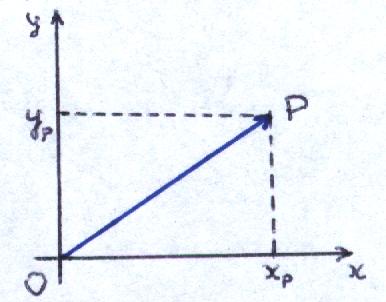
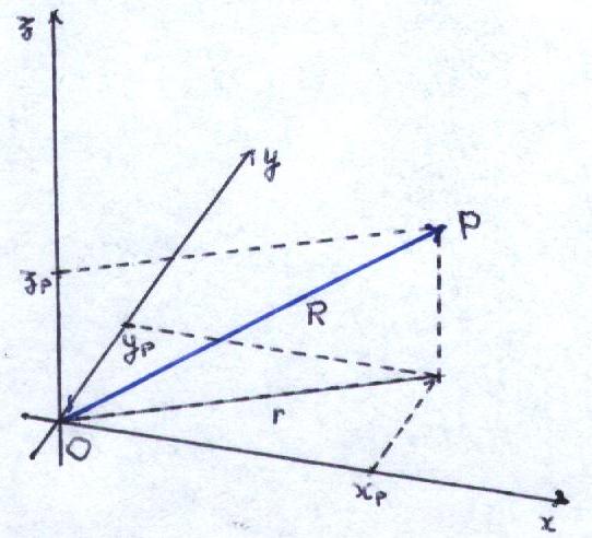
In uno spazio ordinario (euclideo), il teorema di Pitagora afferma che, dato un triangolo rettangolo AOB, retto in O, vale la seguente relazione tra l'ipotenusa AB e i cateti OA e OB:

AB² = OA² + OB².

Questo è facilmente applicabile ad uno spazio a due dimensioni per calcolare il quadrato della distanza di un punto P di coordinate x_P e y_P dall'origine O (vedi grafico).

Il teorema di Pitagora fornisce per il quadrato della distanza r = OP il valore:

(7.1): r² = x_P² + y_P².

Naturalmente, il teorema è estendibile a spazi di qualunque dimensione. Infatti, data una terza dimensione z, si può applicare il teorema dapprima alle coordinate x_P e y_P ed ottenere r, e poi applicarlo a r e alla coordinata z ed ottenere:

R² = r² + z_P² = x_P² + y_P² + z_P².

Sia r che R possiedono un'interessante proprietà. Se applichiamo una rotazione attorno ad un asse, la loro lunghezza non cambia. Perciò essi sono invarianti rispetto alle rotazioni. Includiamo adesso il tempo. Consideriamo un punto di coordinate (t, x, y, z) e poniamo per definizione s² = c² · t² + x² + y² + z² (è necessario introdurre la velocità della luce c per ottenere la corretta dimensione). Domanda: è s² invariante rispetto alle trasformazioni di Lorentz? La risposta è no, come si può verificare facilmente. Allora sorge la seguente domanda: esiste una generalizzazione del teorema di Pitagora che risulti invariante rispetto alle trasformazioni di Lorentz? In questo caso la risposta è sì. Vediamo come funziona.

Limitiamoci per semplicità alle due dimensioni (t, x), consideriamo la seguente espressione

(7.2): s² = c² · t² – x²,

e applichiamo la seguente trasformazione di Lorentz:

t' = ( t + x · v / c² ) · γ, x' = ( x + v · t ) · γ.

I quadrati di t' e x' sono:

t'² = ( t² + 2 · t · x · v / c² + x² · v² / c⁴ ) · γ²,

x'² = ( x² + 2 · x · v · t + v² · t² ) · γ².

Espressa in termini delle nuove coordinate, l'equazione (7.2) diventa (le parti in rosso si cancellano a vicenda):

c² · t'² – x'² =

= ( c² · t² + 2 · t · x · v + x² · v² / c² ) · γ² – ( x² + 2 · x · v · t + v² · t² ) · γ²

= ( c² · t² – x² + x² · v² / c² – v² · t² ) · γ²

= [ c² · t² – x² – v² · ( t² – x² / c² ) ] · γ²

= [ c² · t² – x² · ( v² / c² ) · ( c² · t² – x² ) ] · γ².

= ( c² · t² – x² )  · ( 1 – v² / c² ) · γ²

= c² · t² – x².

L'ultimo passo è conseguenza del fatto che, secondo la definizione, risulta γ² = 1 / ( 1 – v² / c² ). Perciò, vediamo che attribuendo al quadrato di c · t un segno opposto a quello delle coordinate spaziali otteniamo una ricetta che dà quantità invarianti rispetto alle trasformazioni di Lorentz. Per quale motivo il segno della coordinata tempo è positivo mentre quello della coordinata spaziale è negativo e non viceversa? In effetti, ciò che si richiede è che le coordinate temporali e spaziali abbiano segni opposti. Che uno assegni il segno positivo oppure negativo alla coordinata tempo dipende dall'intervallo in considerazione. Per convenienza si dovrebbe scegliere il segno che rende positivo l'invariante s², in modo che la sua radice quadrata risulti reale. Perciò il coefficiente del quadrato degli intervalli di tipo tempo dovrebbe essere positivo, mentre nel caso degli intervalli di tipo spazio il segno positivo dovrebbe essere posto davanti alle parti spaziali. Non è coinvolto niente di fisico; si tratta semplicemente di un requisito matematico necessario per rendere reale la radice quadrata.

Che significato ha l'invariante così definito? Supponiamo che sia di tipo spazio. Allora esiste una trasformazione di Lorentz in grado di rendere nulla la coordinata temporale t'. In tali coordinate abbiamo: s² = x'². Ciò mostra che s rappresenta la distanza spaziale nel sistema in cui t' = 0. Similmente, se x' = 0, s rappresenta l'intervallo temporale nel sistema in cui x' = 0.

Ed ora veniamo alla metrica. Consideriamo di nuovo l'equazione (7.1), ma applichiamo alle coordinate x e y una trasformazione arbitraria. Allora, naturalmente, tale equazione può non essere più valida. Chiediamoci: è possibile avere un'espressione per r² che sia valida in qualsiasi sistema di coordinate? La matematica mostra che la soluzione consiste nel considerare la somma di tutte le combinazioni di x², y², e x · y con appropriati coefficienti, del tipo:

(7.3): r² = g₁₁ (x¹)² + g₁₂ x¹ x² + g₂₁ x² x¹ + g₂₂ (x²)².

Così definiti, i coefficienti g_ij (i, j = 1, 2) prendono il nome di tensore metrico dello spazio a due dimensioni (x, y). Con questo trucco si può calcolare il quadrato delle distanze in (quasi) qualsiasi sistema di coordinate. Questa espressione può essere considerata come la generalizzazione del teorema di Pitagora in uno spazio ordinario (euclideo). Domanda: si applica una formula di questo tipo anche allo spazio-tempo? Sì, purché in un sistema di coordinate ortogonali la formula torni ad essere del tipo espresso dall'equazione (7.2). Una metrica che acquisti la forma (7.2) quando gli assi sono ortogonali è detta minkowskiana. Nella metrica di Minkowski, l'equazione (7.2) prende questa forma:

(7.4): s² = η₀₀ (x⁰)² + η₀₁ x⁰ x¹ + η₁₀ x¹ x⁰ + η₁₁ (x¹)².

In questo caso si è applicato un nuovo simbolo, η_μν. É il simbolo usato generalmente nella letteratura per rappresentare la metrica di Minkowski (la lettera greca η si pronuncia 'eta'). Per mantenere le corrette dimensioni, x⁰ sostituisce c · t. Perché ho usato per le coordinate i simboli x¹, x² e x⁰ invece di x, y e c · t? Per il fatto che con questa notazione si possono applicare alle equazioni (7.3) e (7.4) le seguenti forme abbreviate:

r² = g_ij xⁱ x^j, i, j = 1, 2,

s² = η_μν x^μ x^ν, μ, ν = 0, 1,

dove è sottintesa la sommatoria su tutti i valori degli indici ripetuti. Questa forma abbreviata è molto utile nel trattare con i vettori ed i tensori.

É da notare un'ultima cosa. Applicate a due qualsiasi vettori, le seguenti espressioni

g_ij xⁱ x^j e

η_μν x^μ x^ν,

producono scalari, cioè i valori che si ottengono effettuando la sommatoria sugli indici non dipendono dal sistema di riferimento, a patto che g_ij e η_μν si trasformino appropriatamente (non tratterò la loro legge di trasformazione, essendo che richiede l'uso dell'analisi differenziale che probabilmente non conosci; e d'altra parte questi articoli sono intesi a considerare principalmente gli aspetti fisici).

Pagina principale

The Minkowski metric

In an ordinary (Euclidean) space, the Pythagoras theorem says that, given a triangle AOB, square in O, the following relation holds between the hypotenuse AB and the sides OA and OB:

AB² = OA² + OB².

This is readily applied in a two dimensional space to get the square of the distance from the origin O of a point P of coordinates x_P and y_P (see graph).

Pythagoras theorem gives for the square of the distance r = OP the value:

(7.1): r² = x_P² + y_P².

Of course, the theorem can be extended to any number of dimensions. In fact, given a third dimension z, one can apply the theorem first to the coordinates x_P and y_P to get r, and then to r and the z coordinate to get:

R² = r² + z_P² = x_P² + y_P² + z_P².

Both r and R have an interesting property. If we apply a rotation about any axis, their lengths do not change. They are invariant under rotations. Now let us include time. Consider a point of coordinates (t, x, y, z), and define s² = c² · t² + x² + y² + z² (the introduction of the speed of light c is necessary to get the correct dimension). Question: is s² invariant under Lorentz transformations? The answer is no, as one can easily verify. Then the following question arises: does there exist a generalization of the Pythagoras theorem that is invariant under Lorentz transformations? In this case, the answer is yes. Let us see how it works.

Let's restrict for simplicity to the two dimensional space (t, x), consider the following expression

(7.2): s² = c² · t² – x²,

and apply the following Lorentz transformation:

t' = ( t + x · v / c² ) · γ, x' = ( x + v · t ) · γ.

The squares of t' and x' are:

t'² = ( t² + 2 · t · x · v / c² + x² · v² / c⁴ ) · γ²,

x'² = ( x² + 2 · x · v · t + v² · t² ) · γ².

Equation (7.2), expressed in terms of the new coordinates, gives (the parts in red cancel out):

c² · t'² – x'² =

= ( c² · t² + 2 · t · x · v + x² · v² / c² ) · γ² – ( x² + 2 · x · v · t + v² · t² ) · γ²

= ( c² · t² – x² + x² · v² / c² – v² · t² ) · γ²

= [ c² · t² – x² – v² · ( t² – x² / c² ) ] · γ²

= [ c² · t² – x² · ( v² / c² ) · ( c² · t² – x² ) ] · γ².

= ( c² · t² – x² )  · ( 1 – v² / c² ) · γ²

= c² · t² – x².

The last step follows from the fact that γ² = 1 / ( 1 – v² / c² ). So, we see that by attributing to the square of c · t a sign opposite to that of the spatial coordinates, we obtain a recipe for getting quantities that are invariant under Lorentz transformations. Why is the sign of the time coordinate positive and that of the space coordinate negative, and not viceversa? Actually, all that is required is that time and spatial coordinates have opposite signs. Whether one assigns a positive or negative sign to the time coordinate depends on the interval one measures. For convenience one should take the sign that makes the invariant s² positive, so that a real number come out of its square root. Hence, the coefficient of the square of the time coordinate should be positive for time-like intervals, while for space-like intervals the positive sign should be put before the spatial parts. Nothing physical is involved in this; it's just the mathematical requirement necessary for the square root to be real.

What is the meaning of the invariant thus defined? Suppose the interval space-like. Then there exists a Lorentz transformation such that the transformed time coordinate t' is zero, and s² = x'². This shows that s represents the spatial distance in the system in which t' = 0. Similarly, if x' = 0, s represents the time interval in the system in which x' = 0.

Now let us consider the metric. Take again equation (7.1), but apply to the coordinates x and y an arbitrary transformation. Then, of course, equation (7.1) may be no more valid. Is it possible to get an expression for r² that is valid in any system of coordinates? Mathematics shows that the solution consists in considering the sum of all combinations of x², y², and x · y, with appropriate coefficients, like:

(7.3): r² = g₁₁ (x¹)² + g₁₂ x¹ x² + g₂₁ x² x¹ + g₂₂ (x²)².

People refer to the set of coefficients g_ij (i, j = 1, 2) as to the metric tensor of the two dimensional space (x, y). By using this trick one is able to calculate the square of a distance in (almost) any coordinate system. This expression may be considered as the generalization of Pythagoras theorem in an ordinary (Euclidean) space. Question: does a formula like this apply also to space-time? Yes, provided that when the system of coordinates is orthogonal the formula reduces to the type expressed by equation (7.2). A metric that reduces to type (7.2) when the axes are orthogonal is said to be Minkowskian. In a Minkowski metric, equation (7.2) is usually takes this form:

(7.4): s² = η₀₀ (x⁰)² + η₀₁ x⁰ x¹ + η₁₀ x¹ x⁰ + η₁₁ (x¹)².

In this case a new symbol, η_μν, has been used. This is the one generally used in the literature to represent the Minkowski metric (the Greek letter η is pronounced 'eta'). In order to preserve the proper dimension, x⁰ stands for c · t instead of just t. Why did I use x¹, x² and x⁰ for the coordinates, instead of x, y and c · t? Because with this notation one can apply to equations (7.3) and (7.4) the following shorter forms:

r² = g_ij xⁱ x^j, i, j = 1, 2,

s² = η_μν x^μ x^ν, μ, ν = 0, 1,

where it is understood that summations are to be applied over the repeated indices. This shorter notation is very useful in dealing with vectors and tensors.

One last thing is to be noted. When applied to any two vectors x and y, the expressions

g_ij xⁱ x^j and

η_μν x^μ x^ν,

produce scalars, that is, when summation over the indices are carried out the two expressions produce values independent of the system of reference, provided that g_ij and η_μν transform in the appropriate way (we are not going to consider how they transform, because it requires the use of differential analysis that perhaps you do not know, while we are mostly interested in physics).

Home

La teoria della relatività

La trasformazione di Lorentz fu introdotta affinché le leggi dell'elettromagnetismo mantenessero la stessa forma in qualsiasi sistema di coordinate inerziali, indipendentemente dalla velocità dell'osservatore. Di conseguenza per qualche tempo ci furono due leggi di trasformazione per passare da un sistema di riferimento ad un altro, una per l'elettromagnetismo e un'altra per tutti gli altri fenomeni fisici. Poi nel 1905 per la prima volta Einstein unificò le leggi di trasformazione affermando che “tutte le leggi della fisica devono essere invarianti rispetto alle trasformazioni di Lorentz.” Quest'affermazione sostituì il principio relativistico di Newton, il quale afferma: “I moti dei corpi inclusi in un dato spazio sono gli stessi tra di loro, sia che lo spazio sia a riposo o che si muova in avanti uniformemente e in linea retta.”

Quali furono le implicazioni di questa innovazione? Consideriamo la seconda legge di Newton:

(8.1): f = m · a.

L'equazione vettoriale afferma che una forza f applicata ad un corpo di massa m produce un'accelerazione a inversamente proporzionale alla massa del corpo (più un corpo è pesante e maggiore è la sua inerzia). Come si comporta l'equazione (8.1) quando si cambia sistema di riferimento? Secondo il principio di relatività di Einstein, i membri dell'equazione devono trasformarsi in armonia con la legge di Lorentz. Qui la forza f è indeterminata. Ovviamente, nello specificarla si deve aver cura che essa abbia le corrette caratteristiche. Ciò che ci interessa maggiormente è il termine alla sua destra, il prodotto di ciò che sembra uno scalare, la massa m, e di ciò che sembra un vettore, l'accelerazione a.

Per definizione uno scalare è un valore indipendente dal sistema di riferimento. In quanto all'accelerazione, secondo la definizione essa esprime la variazione della velocità rispetto al tempo, cioè, se Δv è la variazione della velocità che ha luogo al tempo t durante un breve intervallo di tempo Δt, allora essa è data da:

(8.2): a = Δv / Δt.

(La lettera maiuscola greca Δ, che si pronuncia 'delta', è spesso usata in fisica e matematica per denotare la variazione o incremento della variabile alla sua destra, così che Δv sta per 'la variazione di v' e Δt per 'la variazione di t'. Nell'usare rapporti come quello di cui sopra la variazione del numeratore è considerata dipendente da quella del denominatore. Per esempio, se un corpo possiede velocità v₁ al tempo t₁ e v₂ un po' più tardi, al tempo t₂, allora le variazioni sono Δv = ( v₂ – v₁ ) e Δt = ( t₂ – t₁ ).)

L'equazione (8.2) mostra che, anche se la velocità dovesse comportarsi correttamente quando è soggetta ad una trasformazione di Lorentz, non sarebbe così per l'accelerazione, perché possiede un tempo al denominatore, il quale produce un fattore γ quando si esegue una trasformazione di Lorentz (tieni presente che nel considerare la differenza Δt = t₂ – t₁ il termine con x scompare). D'altra parte, la velocità è la variazione dello spazio rispetto al tempo:

v = Δx / Δt.

Qui il numeratore è veramente un vettore, ma la velocità rappresentata dal rapporto non lo è, perché c'è una coordinata tempo al denominatore. In conclusione, né l'accelerazione né la velocità si comportano correttamente rispetto alle trasformazioni di Lorentz. Sebbene siano entrambe caratterizzate da componenti relative ad assi, esse non si comportano come vettori quando sono soggette a trasformazioni di Lorentz. Tuttavia l'equazione (8.1) esprime indubbiamente una buona legge fisica. Come può essa funzionare in qualsiasi sistema di riferimento, essendo che le trasformazioni di Lorentz producono due γ al denominatore? La soluzione deve implicare qualche considerazione fisica.

Diamo all'equazione (8.1) un'altra forma. In fisica esiste un ben noto vettore denominato quantità di moto, il quale è il prodotto massa per velocità:

p = m · v.

In accordo con la definizione, poiché la massa non dipende dal tempo, il membro di destra dell'equazione (8.1) può essere inteso come la variazione della quantità di moto p rispetto al tempo. Infatti:

(8.3): f = m · a

= m · Δv / Δt

= Δ( m · v ) / Δt

= Δp / Δt.

Questa modifica non è di alcun aiuto, a meno che non si possa dimostrare che la quantità di moto p si comporta come un vettore rispetto alle trasformazioni di Lorentz. Come può essere, visto che la velocità contenuta nella sua definizione non è un vero vettore? Il solo modo di soddisfare questo requisito è di ammettere che la massa non sia un vero scalare. Definendo la massa nel modo seguente:

m = m · γ.

il fattore γ della massa neutralizza quello derivante dalla velocità. Poiché γ è uguale ad uno quando la velocità è zero, lo scalare m rappresenta la massa a riposo, cioè la massa che il corpo possiede quando è fermo.

Consideriamo adesso l'ultimo γ. Einstein lo eliminò affermando che il tempo al denominatore dovrebbe essere sostituito dal tempo proprio τ = t / γ, il cui valore, in accordo con la definizione, è indipendente dal sistema di riferimento. Infatti, poiché t' = γ · t, allora

τ' = t' / γ = ( γ · t ) / γ = τ.

cioè, τ' = τ. Sostituendo t con τ, l'equazione (8.3) diventa:

f = Δp / Δτ,

che è chiaramente invariante rispetto alle trasformazioni di Lorentz ed ha perciò la stessa forma in qualsiasi sistema di riferimento.

Con la nuova definizione la massa m non è più uno scalare. Ciò appare piuttosto strano, essendo che essa è sempre stata considerata una proprietà invariante della materia, indipendente dal sistema di riferimento. Ora vediamo invece che a motivo di γ il suo valore è funzione della velocità.

Pagina principale

The theory of relativity

The Lorentz transformation was introduced in order that the electromagnetic laws maintained the same appearance in any inertial frame of coordinates, independently from the velocity of the observer. Consequently, at that time there existed two transformation laws for passing from one system of reference to another, one for the electromagnetic and another one for all the other physical phenomena. Then, in 1905, for the first time Einstein unified all the transformations laws by stating that “all laws of physics must be invariant under Lorentz transformations.” This statement replaced the Newton's principle of relativity, which said: “The motions of bodies included in a given space are the same among themselves, whether that space is at rest or moves uniformly forward in a straight line.”

What did this innovation imply? Consider Newton's second law:

(8.1): f = m · a.

The vector equation states that a force f applied to a body of mass m produces an acceleration a inversely proportional to the mass of the body (massive objects possess greater inertia). How does equation (8.1) behave when subject to a change of reference? According to Einstein's principle of relativity, both sides of the equation should transform according to the Lorentz law. Here the force f is unspecified. Obviously, in specifying it, care must be taken in order that it behave correctly. What interests us most is the term at its right, the product of what looks like a scalar, the mass m, and what looks like a vector, the acceleration a.

By definition a scalar is a value independent of the system of reference. As for the acceleration, according to definition it expresses the variation of velocity with respect to time, that is, if Δv is the variation of velocity at the time t during a small time interval Δt, than the acceleration is:

(8.2): a = Δv / Δt.

(The capital Greek letter Δ, pronounced 'delta', is often used in physics and mathematics to denote variation or incrementation of the variable at its right, so Δv stands for 'the variation of v', and Δt for 'the variation of t'. When ratios like those written above are used, the variation at the numerator is considered dependent on the one at the denominator. For example, if a body has velocity v₁ at the time t₁, and v₂ a little later, at a time t₂, then the variations are Δv = ( v₂ – v₁ ) and Δt = ( t₂ – t₁ ).)

Equation (8.2) shows that even if the velocity behaved correctly under Lorentz transformations the acceleration would not, because it possessed a time at the denominator, which would produce a γ when subject to a Lorentz transformation (keep in mind that in taking the difference Δt = t₂ – t₁ the x term disappears). On the other hand velocity is the variation of space with respect to time:

v = Δx / Δt.

Here, while the numerator is indeed a vector, the velocity represented by the above ratio isn't, because there's a time coordinate at the denominator. In conclusion, neither acceleration, nor velocity behave correctly under Lorentz transformations. Although they're both characterized by components with respect to some axes, they do not act like vectors under Lorentz transformations. Nonetheless, equation (8.1) is undoubtedly a good physical law. How can it work in any frame, while having two γs at the denominator? The solution must involve some physical considerations.

Let us give equation (8.1) another form. In physics there exists a well known vector called momentum, which is the product of mass times velocity:

p = m · v.

According to definition, since the mass does not depend on t the right hand side of equation (8.1) can be thought as the variation with time of the momentum p:

(8.3): f = m · a

= m · Δv / Δt

= Δ( m · v ) / Δt

= Δp / Δt.

This modification is of no help unless we can prove that the momentum p behaves like a vector under Lorentz transformations. How can it be, having seen that the velocity that is part of its definition isn't a true vector? The only way to satisfy this requirement is to admit that the mass isn't a true scalar. By defining the mass in the following way:

m = m · γ.

the γ factor of the mass neutralizes the one associated to the velocity. Since γ is equal to one when the velocity is zero, the scalar m represents the rest mass, that is, the mass the body possesses at rest.

Consider now the last γ. Einstein took care of it by saying that the time at the denominator should be replaced by the proper time τ: = t / γ:. whose value, according to definition, is frame independent. In fact, since t' = γ · t, then

τ' = t' / γ = ( γ · t ) / γ = τ.

that is, τ' = τ, as stated. By substituting t with τ, equation (8.3) becomes:

f = Δp / Δτ,

which is clearly invariant under Lorentz transformations and looks the same in any inertial frame of reference.

With its new definition the mass m is no longer a scalar. This looks quite odd since it had always been considered an invariant property of matter, independent of the system of reference. Now we see instead that through γ its value is velocity dependent.

Home

La massa relativistica

Nel capitolo precedente abbiamo visto che, affinché la seconda legge di Newton sia invariante rispetto alle trasformazioni di Lorentz, la massa deve essere funzione della velocità mediante il fattore relativistico γ:

m = m · γ.

Che cosa significa? Esaminiamo come varia la massa in funzione della velocità. Per velocità ordinarie (v / c << 1) il fattore γ differisce di poco dall'unità e produce un'alterazione molto piccola. Perciò possiamo scrivere la massa come somma della massa a riposo m più un piccolo termine Δm:

(9.1): m · γ = m + Δm.

Se v / c è molto piccolo, allora pure Δm è molto piccolo e possiamo approssimare il calcolo ignorando il quadrato di v / c, di Δm, come pure le loro potenze di grado superiore ed i mutui prodotti del tipo ( v / c ) · Δm. Infatti, se assumiamo che v rappresenti 100 km/h, allora v / c è circa un decimo di milionesimo e v² / c² è dell'ordine di un centesimo di trilionesimo. I termini dell'ordine di grandezza del trilionesimo si possono sicuramente trascurare. Premesso questo, consideriamo la definizione di γ:

γ = 1 / √( 1 – v² / c² ),

e applichiamola all'equazione (9.1). Poiché non vogliamo trattare con radici quadrate, eleviamo a quadrato entrambi i membri. Otteniamo quanto segue:

m² / ( 1 – v² / c² ) = m² + 2 · m · Δm + ... ,

dove i puntini stanno al posto dei termini trascurati. Ora moltiplichiamo entrambi i membri per 1 – v² / c² ed eliminiamo il denominatore, essendo che per v > 0 è diverso da zero. Otteniamo:

m² = m² – m² · ( v / c )² + 2 · m · Δm + ... .

Poiché le parti in rosso si cancellano, un'ulteriore arrangiamento e semplificazione produce:

Δm = ½ · m · v² / c².

A parte la costante c² al denominatore del secondo membro, Δm non è altro che l'energia cinetica di un corpo caratterizzato da massa m e velocità v. Introduciamo questo risultato nell'equazione (9.1) e moltiplichiamo entrambi i membri per c². Otteniamo:

m · c² = m · c² + energia cinetica.

Da questa espressione comprendiamo che E = m · c² rappresenta l'energia totale del corpo e che E = m · c² è la sua energia a riposo. Il principio di relatività, cioè il requisito che tutte le leggi della fisica siano invarianti rispetto alle trasformazioni di Lorentz produce il risultato che tutta la materia possiede energia a riposo e che massa ed energia rappresentano la stessa proprietà fisica (la costante c² cambia essenzialmente solo l'unità di misura).

Ora la domanda è: se la massa, o energia, non è uno scalare, che cos'è? Per rispondere a questa domanda dobbiamo considerare quanto segue. In La teoria della relatività abbiamo visto che grazie alla trasformazione della massa mediante il fattore γ la quantità di moto p = m · v manifesta il corretto comportamento quando è soggetta a trasformazioni di Lorentz. Ora consideriamo una particella a riposo (v = 0). Allora anche p = m · v = 0. Se assoggettiamo la particella ad una trasformazione di Lorentz con velocità v lungo la direzione x¹, la fisica ci dice che essa acquista quantità di moto:

(9.2): p₁' = m · v.

D'altra parte, la legge di Lorentz dice che:

(9.3): p₁' = ( p₁ + p₀ · v / c² ) · γ

Poiché stiamo considerando una particella inizialmente a riposo (p₁ = 0), allora l'equazione (9.3) si riduce a:

(9.4): p₁' = p₀ · γ · v / c²

Dal confronto di (9.2) e (9.4) e usando la (9.1) otteniamo:

m · γ = p₀ · γ / c².

Eliminando il fattore γ otteniamo m = p₀ / c². Perciò, data la relazione esistente tra massa ed energia, possiamo anche scrivere E = p₀. Il risultato è che l'energia rappresenta la componente temporale del quadrivettore p_μ, e la massa, essendo proporzionale all'energia, si trasforma pure come una componente temporale di quadrivettore. É per tale motivo che le è associato il fattore γ. Da ora poi ci riferiremo a p_μ come al quadrivettore energia-quantità di moto.

Pagina principale

The relativistic mass

In the preceding chapter we saw that in order that Newton's second law be invariant under Lorentz transformations the mass had to be velocity-dependent through the relativistic factor γ:

m = m · γ.

What does it mean? Let's examine the deviation produced by velocity to the mass. For ordinary velocities (v / c << 1), the γ factor differs very little from unity, and produces a very small alteration. Hence we can write the mass as the sum of the rest mass m plus a small term Δm:

(9.1): m · γ = m + Δm.

If v / c is very small, then also Δm is very small, and we can approximate the calculations by neglecting the squares of v / c and Δm as well as their powers and the mutual products of the type ( v / c ) · Δm. In fact, if we take v to represent 100 km/h, v / c is about one tenth of a millionth and v² / c² is of the order of one hundredth of a trillionth. The approximation is surely justifiable. Consider now the definition of γ:

γ = 1 / √( 1 – v² / c² ),

and apply it to equation (9.1). Since we do not want to deal with square roots, we square both sides of the resulting equation. Here's what we get:

m² / ( 1 – v² / c² ) = m² + 2 · m · Δm + ... ,

where the dots stand for the neglected terms. Now we multiply both sides by 1 – v² / c² and eliminate the denominator, since for v > 0 it is different from zero. We obtain:

m² = m² – m² · ( v / c )² + 2 · m · Δm + ... .

Since the parts in red cancel out, a further rearrangement and simplification gives:

Δm = ½ · m · v² / c².

Apart from the constant c² at the denominator of the second term, Δm is nothing but the kinetic energy of a body characterized by rest mass m and velocity v. Introduction into equation (9.1) and multiplication of both sides by c² gives:

m · c² = m · c² + kinetic energy.

From here we understand that E = m · c² represents the body's total energy and that E = m · c² is its rest energy. The principle of relativity, i.e., the requirement that all laws of physics be invariant under Lorentz transformations brings forth the result that all matter possesses rest energy and that mass and energy represent the same physical property (the constant c² essentially changes only the unit).

Now the question is: if mass, or energy, is not a scalar, what is it? To answer to this question we must consider what follows. In The theory of relativity we saw that, thanks to the mass transformation property (factor γ) the momentum p = m · v manifests the correct behaviour when subject to Lorentz transformations. Now consider a particle at rest (v = 0). Then also p = m · v = 0. If we subject the particle to a Lorentz transformation with velocity v along the x¹ direction, ordinary physics tells us that the particle acquires the momentum:

(9.2): p₁' = m · v.

However, the Lorentz law says that:

(9.3): p₁' = ( p₁ + p₀ · v / c² ) · γ

Since we are dealing with a particle initially at rest (p₁ = 0), then equation (9.3) reduces to:

(9.4): p₁' = p₀ · γ · v / c²

By comparing (9.2) and (9.4) and using (9.1) we obtain

m · γ = p₀ · γ / c².

By eliminating the γ factor we obtain m = p₀ / c². Hence, given the relationship between mass and energy, we can also write E = p₀. The result is that energy represents the time component of the 4-vector p_μ, and the mass, being proportional to the energy, also transforms like the fourth component of a 4-vector, and for that reason it has a γ factor. From now on we shall refer to p_μ as to the energy-momentum 4-vector.

Home

Il significato della dilatazione del tempo

Fino a questo momento abbiamo considerato la materia secondo il punto di vista particellare. Una migliore conoscenza richiede la comprensione delle sue caratteristiche quantiche e ondulatorie. Ciò apparve evidente sin dall'inizio del secolo scorso quando diversi esperimenti mostrarono al di là di ogni dubbio che la materia possiede proprietà quantiche. Con lo sviluppo della meccanica quantistica (o meccanica ondulatoria, come venne inizialmente definita) la veduta classica della fisica dovette essere radicalmente modificata. Tentare di spiegare la meccanica quantistica va al di là dello scopo di questi scritti, ma vi sono dei semplici fenomeni degni di nota, i quali possono far luce su alcuni aspetti interessanti della fisica moderna. Da questo momento in poi ci concentreremo sulle proprietà ondulatorie della materia e ne esamineremo alcune sue conseguenze.

Secondo la meccanica ondulatoria a ciascuna particella è associata un'onda, la cui frequenza e il numero di onde per unità di lunghezza sono proporzionali all'energia e alla quantità di moto della particella. Le relazioni sono le seguenti:

(10.1): E = h · ν, p = h · n,

dove h è la costante di Planck, ν (pronuncia 'nu') la frequenza dell'onda, e il vettore n rappresenta il numero di onde per unità di lunghezza. La lunghezza del vettore n, n, sta in relazione alla lunghezza d'onda λ (pronuncia 'lambda') nella seguente maniera:

n = 1 / ν.

Di solito nella letteratura al posto della (10.1) si usa la seguente forma alternativa:

E = h · ω, p = h · k.

Qui h = h / ( 2 · π ), e ω = 2 · π · ν (pronuncia 'omega') è pure chiamata frequenza, anche se non rappresenta effettivamente una frequenza ma è proporzionale ad essa, e k = 2 · π · n è chiamato vettore di propagazione. Questa è una piccola inconvenienza diventata comune. Nel seguito aderiremo ad essa. Chiaramente, come il 4-vettore energia-quantità di moto (E, p) a cui sono proporzionali, (ν, n) e (ω, k) sono pure 4-vettori. Ciò che ci interessa di questi nuovi simboli è il loro significato. Come abbiamo visto dalle loro definizioni, le lunghezze n e k sono inversamente proporzionali alla lunghezza dell'onda associata alla particella. A loro volta, ν e ω sono inversamente proporzionali al periodo T:

ν = 1 / T, ω = ( 2 · π ) / T.

Essendo un 4-vettore, (ω, k) ubbidisce alle stesse leggi di trasformazione di (t, x). Ciò comporta un'interessante conseguenza. Esaminiamo come le componenti temporali di questi 4-vettori trasformano nel caso in cui inizialmente le coordinate abbiano l'origine sulla particella stessa (x = 0) la particella si muova lungo la coordinata temporale, cioè il riferimento sia tale che la particella sia ferma (k = 0). In tal caso, le leggi di trasformazione producono semplicemente una moltiplicazione per γ:

t' = t · γ, ω' = ω · γ.

Riguardo al periodo T, che è inversamente proporzionale a ω, abbiamo:

T' = T / γ.

Consideriamo adesso il seguente prodotto:

(10.2): τ = T · t,

(τ si pronuncia 'tau') e applichiamogli una trasformazione di Lorentz:

τ' = T' · t' = ( T / γ ) · ( t · γ ) = T · t = τ.

L'interessante risultato è che τ è invariante rispetto alle trasformazioni di Lorentz. Che cosa significa?

Poiché t rappresenta un intervallo di tempo, così lo è τ. Cosa più importante, dato il significato di T quale periodo d'onda e la definizione (10.2), si comprende che t non è altro che il numero di periodi corrispondenti al tempo invariante τ. Quando si effettua un cambiamento di riferimento, il tessuto dello spazio-tempo non viene dilatato, come la dilatazione del tempo aveva portato a pensare, ma cambiano solo le lunghezze dei periodi ed il loro numero, di modo che il prodotto T · t continua a rappresentare il medesimo tempo invariante τ. Inoltre, poiché le trasformazioni di Lorentz si applicano a qualsiasi particella, i cambiamenti di coordinate influenzano tutte le particelle e tutti gli orologi nella stessa proporzione. Ciò spiega il motivo per cui un cambiamento di coordinate, qualcosa che può essere puramente intellettuale, produce un cambiamento delle lunghezze degli intervalli di spazio e di tempo. Il numero di periodi dipende dalla direzione della linea del tempo nello spazio-tempo quadridimensionale. Come la linea temporale si inclina, viene a modificarsi anche il numero di periodi, e di conseguenza cambia il tempo associato. I cambiamenti non riguardano il tessuto dello spazio-tempo, ma solo le unità di tempo rappresentate dai periodi delle onde, e tutti gli orologi vengono aggiustati secondo le nuove unità. Nella stessa maniera, le lunghezze rappresentano numeri di onde. Un cambiamento di coordinate non altera le effettive lunghezze dell'etere, ma solamente le unità di lunghezza. Ciò dà nuovo credito al concetto di etere e spiega la ragione per cui la materia possiede inerzia, indipendentemente dalla presenza di particelle o campi. In seguito esamineremo questi aspetti in maggiore dettaglio.

Nei capitoli precedenti derivammo le leggi di dilatazione del tempo, contrazione dello spazio e trasformazione di Lorentz dal fatto che la velocità della luce è indipendente dal sistema di riferimento. Ora vediamo che la velocità della luce non è all'origine di ogni cosa, ma come il resto non è altro che una conseguenza delle proprietà di trasformazione delle onde dell'etere rispetto ad un cambiamento di riferimento. Infatti, sono queste le cause primarie e da esse si può derivare ogni altra cosa, inclusa la costanza della velocità della luce. Di conseguenza, sembra che la struttura dell'etere sia molto più complicata di quanto non appaia dal solo studio del tensore metrico e che si sia giunti ad una nuova frontiera nella conoscenza dell'universo in cui viviamo.

Pagina principale

The meaning of the time dilation

Up to now we have considered matter from the particle point of view. A more comprehensive knowledge of it requires the understanding of its quantum and wave-like features. This became apparent at the beginning of last century when several experiments showed without doubt that matter possessed quantum properties. The classical view of physics had to be radically modified and quantum mechanics (or wave mechanics, as was originally called) was developed. Trying to explain quantum mechanics goes beyond the scope of these writings, but there are some simple phenomena worth considering that can shed light on some interesting aspects of modern physics. From now on we shall concentrate on the wave properties of matter and see some consequences that result from them.

According to quantum mechanics, to each particle is associated a wave, whose frequency and number of waves per unit of length are proportional to the energy and momentum of the particle. The relationships are the following:

(10.1): E = h · ν, p = h · n,

where h is Planck's constant, ν (pronunciation 'nu') the frequency of the wave and the vector n represents the number of waves per unit of length. The length of the vector n, n, is related to the wavelength λ (pronounced 'lambda') by

n = 1 / ν.

Most often, instead of (10.1) in the literature people use the following alternative form:

E = h · ω, p = h · k.

Here h = h / ( 2 · π ), ω = 2 · π · ν (pronunciation 'omega') is called frequency, even though it does not really represent a frequency but is proportional to it, and k = 2 · π · n is called the propagation vector. This is a little inconvenience that has become common. In the following we shall adhere to it. Clearly, like the energy-momentum 4-vector (E, p) to which they are proportional, (ν, n) and (ω, k) are also a 4-vectors. What interests us of these new symbols is their meaning. As we have seen from their definitions, the lengths of n and k are inversely proportional to the wavelength of the particle wave. On their part, ν and ω are inversely proportional to the period T:

ν = 1 / T, ω = ( 2 · π ) / T.

Being a 4-vector, under Lorentz transformations (ω, k) transforms like (t, x). This has an interesting consequence. Let us examine how the time-like components of both 4-vectors transform, starting from the situation in which the coordinates have their origin on the particle itself (x = 0), and the particle moves along the time coordinate, i.e. in the frame in which the particle is at rest (k = 0). The transformation laws are then nothing but a simple multiplication by the factor γ:

t' = t · γ, ω' = ω · γ.

Regarding the period T, which is inversely proportional to ω, we have:

T' = T / γ.

Now, consider the product:

(10.2): τ = T · t,

(τ is pronounced 'tau') and apply to it a Lorentz transformation:

τ' = T' · t' = ( T / γ ) · ( t · γ ) = T · t = τ.

The interesting result is that τ is invariant under Lorentz transformations. What does it mean?

Since t represents an interval of time, so is τ. More importantly, given the meaning of T as period of the wave and the definition (10.2) we understand that t is nothing but the number of periods corresponding to the invariant time τ. When a change of reference is made, the texture of space-time isn't stretched, as the time dilation brought to believe, but only the lengths of the periods and their numbers are changed, in order that the product T · t represent the invariant time interval τ. Furthermore, since the Lorentz transformations apply to any particle, a change of coordinates affects all particles and clocks in the same proportion. This explains why a change of coordinates, something one can merely think about, changes the lengths of the space and time intervals. The number of periods depends on the direction of the time line in the four-dimensional space-time. As the time-line is bent, the number of periods is modified, and so is the associated time. The changes themselves don't affect the texture of space-time, but only the time units represented by the periods of the waves, and all clocks are adjusted to the new units. In the same way, lengths represent number of waves. A change of coordinates doesn't alter the true ether lengths, but just the length units. This gives new credit to the concept of ether and explains why matter possesses inertia, independently from the presence of particles or fields. Later on we shall examine these aspects in more detail.

In the previous chapters we derived the laws of time dilation, space contraction and the Lorentz transformation from the fact that the speed of light is independent of the frame of reference. Now we see that the speed of light isn't the cause of everything, but, like the rest, just a consequence of the transformation properties of the ether waves under a change of reference. In fact, this is the primary cause, and from it one can derive everything else, including the constancy of the speed of light. Hence, it seems that the ether structure has to be much more complicated than what appears from the sole study of its metric tensor and that we've arrived at a new frontier in the knowledge of the universe we live in.

Home

Corrispondenza tra l'etere e l'universo fisico

Nel capitolo precedente abbiamo visto come le lunghezze spaziali e temporali dipendono dalle lunghezze e dai periodi delle onde, mentre il tessuto dell'etere non è modificato dal cambiamento della direzione temporale. Ora considereremo la relazione che esiste tra un insieme di coordinate relative all'etere (le chiamiamo x^μ) e le corrispondenti coordinate dell'universo fisico (che chiamiamo y^ν). Poiché le lunghezze dell'etere non sono influenzate dalle rotazioni che coinvolgono l'asse temporale, la metrica deve essere ordinaria euclidea, ossia in un sistema di coordinate ortogonali il quadrato della distanza dall'origine ad un punto P, caratterizzato dal vettore (x⁰, x¹, x², x³) deve essere data dal teorema esteso di Pitagora:

(11.1): s_x² = ( x⁰ )² + ( x¹ )² + ( x² )² + ( x³ )²,

mentre nello spazio-tempo fisico lo stesso quadrato espresso in termini del vettore corrispondente (y⁰, y¹, y², y³) deve avere la forma minkowskiana:

(11.2): s_y² = ( y⁰ )² – ( y¹ )² – ( y² )² – ( y³ )²,

se l'intervallo è di tipo tempo, oppure:

(11.3): s_y² = ( y⁰ )² + ( y¹ )² + ( y² )² – ( y³ )²,

se è di tipo spazio. Le equazioni (11.2) e (11.3) si possono unificare in un'unica espressione nel modo che segue:

(11.4): s_y² = | ( y⁰ )² – ( y¹ )² – ( y² )² – ( y³ )² |,

dove le barre verticali significano che al valore dell'espressione contenuta nel loro interno deve essere attribuito il segno positivo.

Usando il formalismo introdotto in La metrica di Minkowski l'equazione (11.1) può essere espressa in forma contratta come segue:

(11.5): s_x² = e_μν x^μ x^ν,

dove e_μν è il tensore metrico dell'etere (si è introdotta una x come pedice della lunghezza s per ricordare che la stiamo esprimendo mediante le coordinate dell'etere), mentre una semplificazione simile dell'equazione (11.4) produce:

(11.6): s_y² = | η_μν y^μ y^ν |,

dove  η_μν è il tensore metrico di Minkowski relativo allo spazio-tempo fisico. Naturalmente si comprende che in entrambi i casi si deve operare la sommatoria sugli indici ripetuti μ e ν. Stabiliamo ora una relazione tra le coordinate dei due spazi.

Consideriamo il caso in cui le coordinate fisiche siano a riposo rispetto all'etere (chiamiamo fondamentale un tale sistema). Se entrambe le coordinate sono ortogonali, allora si possono far coincidere, e in tal caso y^μ = x^μ.

Supponiamo di sottoporre le coordinate fisiche ad una trasformazione di Lorentz: y^μ' = L^μ_ν x^ν, dove L^μ_ν è la matrice che esprime tale trasformazione. In particolare, se il moto avviene lungo l'asse x¹, con velocità v, allora:

(11.7): y⁰' = ( x⁰ + v ∙ x¹ / c ) ∙ γ ,

(11.8): y¹' = ( x¹ + v ∙ x⁰ / c ) ∙ γ ,

dove γ = 1 / √( 1 - v² / c² ), mentre le altre coordinate rimangono inalterate.

Consideriamo adesso gli assi delle nuove x^μ' e siano che rimangano paralleli a quelli delle y^μ'. Essi non sono più ortogonali, ma si deve richiedere che siano preservate le unità di riferimento. Nell'etere, le trasformazioni che corrispondono a quelle delle coordinate fisiche sono le seguenti:

(11.9): x⁰' = x⁰ ∙ cos( θ ) + x¹ ∙ sen( θ ),

(11.10): x¹' = x¹ ∙ cos( θ ) + x⁰ ∙ sen( θ ),

dove θ = arctan( v / c ), cos( θ ) = 1 / √( 1 + v² / c² ), sen( θ ) = ( v / c ) / √( 1 + v² / c² ). Ciascun asse è soggetto ad un'ordinaria rotazione, ma in direzioni opposte, così che entrambi i termini che contengono la funzione sen( θ ) hanno lo stesso segno, positivo o negativo, a seconda della direzione della rotazione.

Espresse in funzione della velocità v, le rotazioni (11.9) e (11.10) hanno la seguente espressione:

(11.11): x⁰' = ( x⁰ + v ∙ x¹ / c ) / √( 1 + v² / c² ),

(11.12): x¹' = ( x¹ + v ∙ x⁰ / c ) / √( 1 + v² / c² ),

con le inverse:

(11.13): x⁰ = ( x⁰' - x¹' ∙ v / c ) ∙ √( 1 + v² / c² ) / ( 1 - v² / c² ),

(11.14): x¹ = ( x¹' - x⁰' ∙ v / c ) ∙ √( 1 + v² / c² ) / ( 1 - v² / c² ).

Introducendo (11.13) e (11.14) in (11.7) e (11.8) si ottiene il seguente risultato:

(11.15): y⁰' = x⁰' ∙ γ ∙ √( 1 + v² / c² ),

(11.16): y¹' = x¹' ∙ γ ∙ √( 1 + v² / c² ),

In conclusione, segliendo appropriatamente gli assi e le unità di misura, in generale esiste la seguente relazione tra le coordinate fisiche e quelle dell'etere:

y⁰ = x⁰ ∙ Γ,

y¹ = x¹ ∙ Γ,

y² = x²,

y³ = x³,

dove Γ = √[( 1 + v² / c² ) / ( 1 - v² / c² )] e v è la velocità del sistema fisico rispetto a quello fondamentale (cioè, quello dell'etere a riposo). Lungo la direzione di moto le lunghezze sono dilatate.

Pagina principale

Correspondence between the ether and the physical universe

In the previous chapter we saw how the lengths in space and time depend on the wavelengths and periods of the waves, while the texture of the ether isn't affected by the changes of the time direction. Now we're going to consider the relationship that exists between a set of coordinates established on the ether (we call them x^μ), and the corresponding ones on the physical universe (which we call y^μ). Since on the ether lengths aren't affected by rotations involving the time axis, the metric has to be ordinary Euclidean, that is, in a system of orthogonal coordinates the square of the distance from the origin to a point P, characterized by the vector (x⁰, x¹, x², x³), has to be given by the extended Pythagoras theorem:

(11.1): s_x² = ( x⁰ )² + ( x¹ )² + ( x² )² + ( x³ )²,

while in the physical space-time the same square in terms of the corresponding vector (y⁰, y¹, y², y³) has the Minkowskian form:

(11.2): s_y² = ( y⁰ )² – ( y¹ )² – ( y² )² – ( y³ )²,

if the interval is time-like, or:

(11.3): s_y² = ( y⁰ )² + ( y¹ )² + ( y² )² – ( y³ )²,

if it is space-like. Equations (11.2) and (11.3) can be combined into a unique expression as follows:

(11.4): s_y² = | ( y⁰ )² – ( y¹ )² – ( y² )² – ( y³ )² |,

where the vertical bars mean that the resulting value of what lies inside them has to be attributed the positive sign.

Using the formalism introduced in The Minkowski metric, equation (11.1) can be expressed in a contracted form, like:

(11.5): s_x² = e_μν x^μ x^ν,

where e_μν is the ether metric tensor (the subscript x is introduced just to remind us that we are dealing with the ether coordinates), while a similar simplification in form of equation (11.4) produces:

(11.6): s_y² = | η_μν y^μ y^ν |,

with η_μν being the Minkowski metric tensor of the physical space-time. Of course, it is understood that in both cases summation is to be carried out over the repeated indices μ, and ν. Now, let us establish a relationship between the coordinates of the two spaces.

Consider the case in which the physical coordinates are at rest with respect to the ether (we call such a system fundamental). If the coordinates are both orthonormal, then they can be made to coincide, and in that case y^μ = x^μ.

Suppose that the physical coordinates be subjected to a Lorentz transformation: y^μ' = L^μ_ν x^ν, where L^μ_ν is the matrix that expresses the transformation. In particular, if the motion occurs along the x¹ direction with velocity v, then:

(11.7): y⁰' = ( x⁰ + v ∙ x¹ / c ) ∙ γ ,

(11.8): y¹' = ( x¹ + v ∙ x⁰ / c ) ∙ γ ,

where γ = 1 / √( 1 - v² / c² ), while the other coordinates remain unchanged.

Consider now the axes of the new x^μ', and require that they be parallel to those of the y^μ'. They are no longer orthogonal, but it must be required that the referencing units be preserved. The corresponding ether transformations are the following:

(11.9): x⁰' = x⁰ ∙ cos( θ ) + x¹ ∙ sin( θ ),

(11.10): x¹' = x¹ ∙ cos( θ ) + x⁰ ∙ sin( θ ),

where θ = arctg( v / c ), cos( θ ) = 1 / √( 1 + v² / c² ), sin( θ ) = ( v / c ) / √( 1 + v² / c² ). Each axis is subject to an ordinary rotation, but on opposite directions, so that both terms with the sin( θ ) have the same sign, either positive or negative, depending on the direction of rotation.

In terms of the velocity v, the above rotations have the following espression:

(11.11): x⁰' = ( x⁰ + v ∙ x¹ / c ) / √( 1 + v² / c² ),

(11.12): x¹' = ( x¹ + v ∙ x⁰ / c ) / √( 1 + v² / c² ),

with inverses:

(11.13): x⁰ = ( x⁰' - x¹' ∙ v / c ) ∙ √( 1 + v² / c² ) / ( 1 - v² / c² ),

(11.14): x¹ = ( x¹' - x⁰' ∙ v / c ) ∙ √( 1 + v² / c² ) / ( 1 - v² / c² ).

Substitution of (11.13) and (11.14) into (11.7) and (11.8) produces the following result:

(11.15): y⁰' = x⁰' ∙ γ ∙ √( 1 + v² / c² ),

(11.16): y¹' = x¹' ∙ γ ∙ √( 1 + v² / c² ),

In conclusion, with appropriately chosen axes and measuring units, the following general relationship exists between the physical and the ether coordinates:

y⁰ = x⁰ ∙ Γ,

y¹ = x¹ ∙ Γ,

y² = x²,

y³ = x³,

where Γ = √[( 1 + v² / c² ) / ( 1 - v² / c² )], and v is the velocity of the physical system with respect to the fundamental one (ether at rest). Along the direction of motion with respect to the ether, the lengths are dilated.

Home

Proprietà dello spazio-tempo

Nel capitolo precedente abbiamo ricavato la relazione esistente tra il tensore metrico dell'etere e quello dell'universo fisico (riguardo alla simbologia, vedi La metrica di Minkowski Corrispondenza tra l'etere e l'universo fisico). Ora consideriamo cosa succede se si cambia sistema di riferimento mediante una rotazione degli assi, oppure passando da un sistema di riferimento inerziale ad un altro in movimento rispetto al primo (i calcoli non verranno riportati). A differenza dello spazio-tempo fisico, l'etere possiede un sistema di riferimento privilegiato, caratterizzato da un volume, o ipersuperficie, di tipo spazio Σ ('sigma') (è preferibile chiamarlo ipersuperficie perché la sua dimensione è di un'unità inferiore di quella dello spazio-tempo fisico), la quale si muove costantemente nella direzione dell'asse positivo del tempo. Ciò definisce in ciascun punto dello spazio-tempo un'unica direzione temporale. Chiamiamo fondamentale qualsiasi sistema di riferimento con quella direzione del tempo. Perciò, nell'etere il concetto di contemporaneità è privo di ambiguità e nel sistema fondamentale i tensori hanno i seguenti valori:

(12.1): e_μν = 1, if μ = ν, e 0 altrimenti,

(12.2): g₀₀ = 1, g_ii = –1 per i = 1, 2, 3,

e zero in tutti gli altri casi

(alternativamente, si possono prendere i segni opposti).

Le equazioni (12.1) e (12.2) definiscono univocamente il sistema fondamentale in ciascun punto dello spazio-tempo a meno di rotazioni puramente spaziali. Se nel sistema fondamentale ruotiamo gli assi spaziali, entrambi i tensori metrici e_μν, g_μν ed il rapporto a (vedi Corrispondenza tra l'etere e l'universo fisico) rimangono inalterati. Questo significa che nel sistema fondamentale sia l'etere che l'universo fisico non possiedono alcun asse spaziale privilegiato, cioè possiedono entrambi la proprietà dell'isotropia.

Consideriamo adesso un sistema di riferimento in moto rispetto al sistema fondamentale. Le trasformazioni di Lorentz non alterano il tensore metrico fisico η_μν, perché esso possiede questa proprietà per definizione. Ciò non è vero nel caso del tensore metrico dell'etere e_μν, perché esso è invariante solo rispetto alle rotazioni ordinarie. Quando si applica una trasformazione di Lorentz, le x^μ si trasformano come le y^μ, essendo il fattore a uno scalare. Di conseguenza, sia la coordinata temporale che quella spaziale nella direzione del tempo appaiono allungate. Ciò non significa che l'etere venga effettivamente dilatato. Significa semplicemente che le nuove unità non rappresentano più fedelmente le lunghezze nell'etere. Tuttavia il tensore metrico dell'etere si prende cura dello stiramento. Infatti, i calcoli mostrano che in un sistema di riferimento che si muove con velocità v lungo l'asse x¹, le componenti del tensore metrico dell'etere divengono (ignoriamo le componenti che rimangono invariate):

(12.3) e₀₀' = e₁₁' = ( 1 + v² / c² ) · γ²,

e₀₁' = e₁₀' = – ( 2 · v / c ) · γ².

Diversamente dal sistema fondamentale, in un sistema in movimento le componenti e₀₁' ed e₁₀' sono diverse da zero. Questo avviene per il fatto che nel nuovo riferimento gli assi non sono più ortogonali. Un altro punto interessante è il fatto che e₀₀' ed e₁₁' non sono più uguali all'unità, il che significa che in questo sistema di riferimento le unità lungo le nuove direzioni non sono quelle naturali. Da questi fatti si comprende che si potessero determinare mediante esperimenti i valori delle e_μν', allora si potrebbe determinare anche la velocità del sistema rispetto all'etere.

Si manifesta l'anisotropia nell'universo fisico? No, perché il tensore metrico di Minkowski è invariante rispetto alle trasformazioni di Lorentz. Tutte le leggi della fisica che sono invarianti rispetto alle trasformazioni di Lorentz non possono rivelare l'anisotropia. Questo fatto fu chiaramente dimostrato dall'esperimento di Michelson e Morley (vedi l' Introduzione alla teoria della relatività). Perciò tutti i fenomeni fisici che ubbidiscono al principio della relatività ristretta manifestano l'isotropia in tutti i sistemi di riferimento inerziali. La sola legge fisica che potrebbe possibilmente rivelare l'anisotropia della spazio-tempo è quella della gravitazione, poiché non è mai stata dimostrata sperimentalmente di essere invariante rispetto alle trasformazioni di Lorentz. A suggerire la sua possibile non-invarianza è il fatto che sembra che la gravitazione non operi mediante onde, come l'elettromagnetismo, ma mediante deformazioni dell'etere. Quindi, per ciò che riguarda la gravitazione le distanze potrebbero non dipendere dalla velocità, ma essere intrinseche dell'etere. Stando così le cose dovrebbe essere possibile determinare i valori delle componenti del tensore metrico dell'etere e, da essi, la velocità della terra rispetto all'etere. Come? Ecco la descrizione di un possibile modo.

Consideriamo un pianeta in orbita attorno al sole. Poiché le distanze eteree non sono influenzate da un cambiamento di riferimento, il suo moto orbitale è in armonia con le leggi fisiche solamente nel sistema fondamentale. Infatti, nel sistema di riferimento fisico le lunghezze appaiono contratte nella direzione del moto e l'orbita appare un poco schiacciata e non in perfetto accordo con le leggi del moto. Nello stesso tempo, la velocità del pianeta subisce delle mutazioni lungo l'orbita per il fatto che il piano di contemporaneità fisico è inclinato rispetto a quello del sistema fondamentale (vedi Contemporaneità in relatività) ed il pianeta impiega minor tempo a muoversi nella direzione del moto dell'universo fisico che in quello opposto, con la variazione dipendente dalla velocità dell'universo fisico rispetto all'etere. Misurando queste variazioni, dell'orbita o delle velocità, si possono calcolare le componenti del tensore metrico dell'etere, e da queste, in base alle equazioni (12.3), ricavare la velocità della terra rispetto all'etere. Una domanda: perché non si sono mai osservate queste discrepanze? La ragione è che sono molto piccole. Tanto per fare un esempio, se la terra si muovesse ad una velocità di 100.000 km/h rispetto all'etere, la deviazione delle componenti del tensore metrico dell'etere sarebbe dell'ordine di 10⁻⁸. Tali piccole deviazioni sono difficili da osservare. Un'altra ragione può essere dovuta al fatto che il sistema solare potrebbe muoversi lungo una direzione pressocché ortogonale al piano dell'eclittica. In tal caso la rilevazione delle discrepanze del tensore metrico richiede l'invio ed il monitoraggio di alcune sonde spaziali.

Pagina principale

Space-time properties

In the previous chapter we derived the relationship between the ether- and the physical metric tensors (for the use of the symbols, examine The Minkowski metric and Correspondence between the ether and the physical universe). Now let's examine what happens if we change system of reference, by rotating the axes or by moving from one inertial system of reference to another one (the calculations will be omitted). Differently from the physical space-time, the ether possesses a privileged system of reference characterized by a space-like volume, or hyper-surface, Σ ('sigma') (we call it hyper-surface because its dimension is one less than that of the physical space-time) that constantly moves along the positive time direction. This defines at each point of space-time a unique time direction. We call fundamental any frame with that time direction. Hence, in the ether the concept of contemporaneity is unambiguous and in the fundamental frame the metric tensors have the following values:

(12.1): e_μν = 1, if μ = ν, and 0 otherwise,

(12.2): g₀₀ = 1, g_ii = –1 for i = 1, 2, 3,

and zero in all the other cases

(alternatively, one can equally well take the opposite signs).

On the other hand, equations (12.1) and (12.2) uniquely define the fundamental frame at each point of space-time up to purely spatial rotations. If we rotate the spatial axes in the fundamental frame, both the metric tensors e_μν, g_μν and the ratio a (see Correspondence between the ether and the physical universe) remain unchanged. This means that in the fundamental frame both the ether and the physical universe don't possess any privileged spatial axis, i.e., they share the property of isotropy.

Now, consider a system of reference that is moving with respect to the fundamental frame. Lorentz transformations don't alter the physical metric tensor η_μν, because it possesses this property by definition. This is not true in the case of the ether metric tensor e_μν, because it's invariant only under ordinary rotations. When a Lorentz transformation is applied, the x^μ transform like the y^μ, since the factor a is a scalar. Consequently, both the time coordinate and the spatial coordinate in the direction of motion appear stretched. This doesn't mean that the ether gets effectively stretched. It simply means that the new units don't faithfully represent the ether lengths. However, the ether metric tensor takes care of the stretching. In fact, a calculation shows that in a system of reference that moves with velocity v along the x¹ axis the components of the ether metric tensor become (we ignore the components that remain unchanged):

(12.3) e₀₀' = e₁₁' = ( 1 + v² / c² ) · γ²,

e₀₁' = e₁₀' = – ( 2 · v / c ) · γ².

Unlike the fundamental frame, in a moving frame the components e₀₁' and e₁₀' are different from zero. This is because in the new frame the axes are no longer orthogonal. Another interesting point is the fact that e₀₀' and e₁₁' are no longer equal to unity, which means that in this frame the units along the new directions aren't the natural ones. From these facts we understand that if it were possible to determine through experiments the values of the e_μνs, then also the velocity of the system with respect to the ether could be derived.

Does anisotropy manifest itself in the physical world? No, because the Minkowski metric tensor is invariant under Lorentz transformations. All laws of physics that are invariant under Lorentz transformations cannot detect anisotropy. This fact was clearly proven by the Michelson and Morley experiment (see Introduction to relativity). Therefore, all physical phenomena that obey to the principle of special relativity manifest isotropy in any inertial frame. The only possible law that might reveal the anisotropy of space-time is the gravitational one, since it has never been experimentally proved to be invariant under Lorentz transformations. To suggest its possible non-invariance is the fact that gravitation does not seem to operate through waves like electromagnetism, but through overall deformations of the ether. Hence, for what concerns gravitation, distances might not be velocity dependent, but intrinsic of the ether. Being this the case, then it should be possible to determine the values of the components of the ether metric tensor, and from them the velocity of the earth with respect to the ether. How? Here's a possible way.

Consider a planet orbiting the sun. Since the ether distances are not affected by a change of reference, its orbit is in agreement with the laws of motion only in the fundamental frame. In fact, in the physical reference the lengths are contracted in the direction of motion and the orbit appears a little flattened and not in perfect agreement with the laws of motion. At the same time, the velocity of the planet appears to vary along the orbit for the reason that, since the physical plane of contemporaneity is bent with respect to that of the fundamental frame (see Contemporaneity in relativity), it takes less time for the cosmic object to move in the direction of motion of the physical universe than in the opposite direction, the variation depending on the velocity of the physical universe with respect to the ether. By measuring these variations, either of the orbit or of the velocity, one is able to calculate the components of the ether metric tensor, and from them, according to equations (12.3), the velocity of the earth with respect to the ether. One question one might ask: why don't these discrepancies have been detected so far? The reason is that they are very small. As an example, if the earth moved with respect to the ether at 100,000 km/h, the deviation of the components of the ether metric tensor would be of the order of 10⁻⁸. Such small deviations are hard to detect. Another reason may be due to the fact that the solar system might move along a direction nearly orthogonal to the ecliptic plane. In such case, the detection of the discrepancies of the metric tensor requires the launch and monitoring of space probes.

Home

L'origine dell'inerzia

Come si è visto in Il significato della dilatazione del tempo, il fatto che la dilatazione dello spazio-tempo sia dovuta alla legge di trasformazione delle onde appoggia l'idea che le onde particellari siano oscillazioni del mezzo che pervade l'intero universo, l'etere. In Corrispondenza tra l'etere e l'universo fisico abbiamo esaminato la relazione che esiste tra lo spazio etereo e quello fisico. Come si deduce l'inerzia dall'esistenza dell'etere? Consideriamo un'onda associata ad una particella. Essa si muove lungo una direzione temporale con frequenza proporzionale alla sua energia, quella indicata dal 4-vettore k^μ = (ω, k), la quale è ortogonale alle sue superfici di fase costante. Un'onda associata ad una particella a riposo ha il vettore k^μ parallelo alla coordinata temporale e si muove in tale direzione. Essa può cambiare direzione di moto nello spazio quadridimensionale solo mediante l'interazione con altre onde, ed infatti si può dire senza andare nei dettagli che le onde particellari si combinano vettorialmente e che i risultati finali sono onde con direzioni di moto cambiate (vedremo meglio questo aspetto quando andremo a considerare in un certo dettaglio Il processo Compton). Per esempio, se k₁^μ e k₂^μ sono i 4-vettori associati a due particelle interagenti, un processo che coinvolga un'interazione tra di loro soddisfa la seguente relazione

k₁^μ + k₂^μ = k₁^μ' + k₂^μ'.

A parte una costante di proporzionalità, essa non è altro che la legge di conservazione dell'energia-quantità di moto, poiché la somma a sinistra è proporzionale all'energia-quantità di moto totale prima dell'interazione e quella a destra all'energia-quantità di moto totale dopo l'interazione. Perciò la conservazione dell'energia-quantità di moto deriva dalla legge di combinazione vettoriale dei quadrivettori che rappresentano le onde. Basilarmente le particelle possiedono inerzia perché in mancanza di interazioni con altre particelle, o campi, il vettore k^μ che rappresenta le superfici delle fasi rimane costante. Perciò, l'etere provvede il riferimento rispetto al quale direzioni e posizioni diverse nello spazio-tempo sono distinguibili e solamente mediante l'interazione con altre particelle o campi una particella può cambiare il suo stato di moto. Infatti, l'elemento chiave che dà origine all'inerzia è la distinguibilità delle diverse posizioni e direzioni di moto nello spazio-tempo provvedute dall'etere. Per questa ragione, l'inerzia è una proprietà locale indipendente dalle posizioni delle stelle fisse, come di solito ci si riferisce nel menzionare il principio di Mach (questo principio fu introdotto da Einstein nel 1918, in riferimento ad un libro scritto nel 1912 da Mach, nel quale questi ragionò riguardo all'influenza delle stelle lontane sul moto di un corpo ruotante). Alcuni scienziati di fama ultimamente hanno messo in dubbio la veracità del principio di Mach.

A questo punto voglio discutere un momentino sul concetto di spazio vuoto, anche se alcune persone potrebbero considerare anatema ciò che andrò a scrivere. Il mio punto di vista è che parlare di distanze non nulle in assenza di qualche specie di etere è privo di significato, perché in tale situazione non ha alcun senso parlare di metrica o di intervalli spazio-temporali. Parlare di vuoto senza il supporto di un mezzo, senza alcuna cosa che stabilisca le distanze e le curvature, che distingua un punto da un altro, ecc., rende privo di significato anche il concetto di particelle, campi, o stelle, perché non c'è niente che possa oscillare, e se non c'è niente che oscilli non ha neppure senso parlare di frequenze e di vettori di propagazione. Inoltre, consideriamo ad esempio due particelle separate da ... niente ed un campo che vada dalla particella 1 alla particella 2. Che significato ha dire che il campo tra le due particelle si propaga alla velocità della luce se non esiste niente che rappresenti spazio e tempo tra di esse? Come può un campo procedere nel niente e qual'è il significato di velocità in esso? Inoltre, se il vuoto è perfetto, non vi è etere, non vi è niente tra le due particelle, non dovrebbero le particelle toccarsi?

Parlare dell'esistenza di qualcosa che non esistre è contradditorio. É vero che esistono teorie di azione a distanza, ma ciò non significa che esse operino in assoluta nullità. Secondo la mia opinione esse trascurano semplicemente il mezzo che separa i diversi oggetti in considerazione, perché non influisce sui processi coinvolti. Quindi non è sbagliato ignorare il mezzo, eccetto quando esso svolge un ruolo. Credo che esistano parecchie leggi della fisica, ovvero migliori spiegazioni di leggi fisiche e principi noti che attendono di essere scoperti. Prendere in considerazione l'esistenza dell'etere e studiarne la struttura può rivelarsi un buon approccio per scoprirli.

Concludo l'argomento riguardo l'etere mettendo in relazione le proprietà di trasformazione del tensore metrico dell'etere e_μν e del rapporto a che è stato trattato in Corrispondenza tra l'etere e l'universo fisico, con isotropia ed inerzia. Abbiamo già visto che l'invarianza del tensore metrico dell'etere rispetto alle rotazioni significa isotropia, cioè significa che le direzioni nella spazio sono indistinguibili. Sottoponiamo ora le coordinate ad una trasformazione di Lorentz. Abbiamo pure già visto che in questo caso il tensore metrico dell'etere non è invariante rispetto ad essa. Quindi l'isotropia non include il tempo e tali trasformazioni producono risultati fisicamente distinguibili. Le trasformazioni fisiche che alterano le direzioni temporali producono un cambiamento dello stato di moto, il quale non può avvenire spontaneamente. In altre parole, l'inerzia è conseguenza della non-invarianza del tensore metrico dell'etere rispetto alle trasformazioni di Lorentz. Tuttavia, qualcuno potrebbe chiedere: perché i corpi manifestano inerzia quando sono soggetti a rotazioni, essendo che il tensore metrico dell'etere è invariante rispetto a tali trasformazioni? La ragione è che i corpi hanno dimensioni finite e quindi le rotazioni implicano dei movimenti.

Un'ulteriore trasformazione di coordinate degna di nota è la traslazione dell'origine degli assi, sia spaziale che temporale. Il tensore metrico dell'etere è invariante rispetto a tali trasformazioni. Riguardo al rapporto a, il suo valore dipende dalla direzione dei raggi che escono dall'origine. Di essi ce ne sono ∞³. Dato un raggio, generalmente una traslazione non lascia invariato il rapporto a ad esso associato. Quindi le diverse posizioni dello spazio-tempo sono distinguibili, ossia ognuna ha la sua individualità entro l'etere. Anche qui si può parlare di inerzia, ma un diverso tipo d'inerzia, nel senso che, anche se è vero che i campi possono traslare solo se soggetti a qualche tipo di interazione, tuttavia in questo caso si comprende che il moto è dovuto all'auto-interazione, come nel caso delle onde del mare che si spostano rinnovandosi costantemente mediante l'energia e la quantità di moto di cui sono dotate. Perciò l'etere possiede una proprietà tale che, anche se non si muove, a parte alcune dilatazioni e rilassamenti temporanei, tale proprietà fa sì che le onde continuino a rinnovarsi, apparentemente senza sforzo o attrito lungo le direzioni ortogonali alle loro superfici di fase costante. Di conseguenza, le equazioni del moto delle onde sono manifestazioni di questa proprietà dell'etere.

Pagina principale

The origin of inertia

As we saw in The meaning of the time dilation, the fact that space-time stretching is due to the wave transformation law supports the idea that particle waves are oscillations of the medium that pervades the whole universe, the ether. In Correspondence between the ether and the physical universe we examined the relationship that exists between the ether space and the physical one. How does the existence of the ether explain inertia? Consider a wave associated to a particle; it moves along a time-like direction with frequency proportional to its energy, the one indicated by the 4-vector k^μ = (ω, k), which is orthogonal to its surfaces of constant phase. A wave associated to a particle at rest has its vector k^μ parallel to the time coordinate and moves in that direction. It can change direction of motion in the 4-dimensional space only through interaction with other waves, and in fact one can say without going into the details that particle waves combine vectorially and that their final results have their directions of motion changed (we'll see better this aspect when we shall consider in some detail The Compton process). For example, if k₁^μ and k₂^μ are the 4-vectors associated to two interacting particles, a process involving an interaction between them satisfies the following relation

k₁^μ + k₂^μ = k₁^μ' + k₂^μ'.

Apart from a constant of proportionality, this is nothing but the energy-momentum conservation law, since the sum on the left is proportional to the total energy-momentum before the interaction and the one on the right to the total energy-momentum after the interaction. Hence, the conservation of energy-momentum derives from the vector combination law of the 4-vectors that represent the waves. Basically, particles possess inertia because without interaction with other particles, or fields, the vector k^μ that represents the phase surfaces remains constant. Hence, the ether provides the reference with respect to which different directions and positions in space-time are distinguishable and only through the interaction with other particles or fields a particle can change its state of motion. In fact, the key element that originates inertia is the distinguishability of the different positions and the directions of motion in space-time provided by the ether. For this reason inertia is a local property, independent from the positions of the fixed stars, as people usually refer to in mentioning Mach's principle (this principle was introduced by Einstein in 1918 in reference to a book written in 1912 by Mach, who had reasoned about the influence of the distant stars on the motion of a rotating body). A few renowned scientists lately questioned the truth of Mach's principle.

At this point I want to digress a little bit about the concept of empty space, even if some people might call anathema what I'm going to write, since vacuum has been considered a perfectly reasonable physical state for about a century, independently from the existence of the ether. My point of view is that speaking of non-null distances in the absence of some sort of ether is meaningless, because in such situation it doesn't have any meaning to talk about metric or space-time intervals. Talking of void without the support of some medium, without anything to establish distances and curvatures, to distinguish one point from another, and so on, renders meaningless also the concepts of particles, fields, or stars, because nothing oscillates, and if nothing oscillates it's also meaningless to speak about frequencies and propagation vectors. Moreover, consider for example two particles separated by ... nothing and a field that goes from particle 1 to particle 2. What does it mean saying that the field between the two particles proceeds at the speed of light, if there's nothing that represent space and time between them? How can a field proceed in nothingness and what's the meaning of velocity in it? Also, if there's a perfect vacuum, no ether, nothing between the two particles, shouldn't the particles touch each other?

Talking of the existence of something that doesn't exist is contradictory. It's true that there are theories of action at a distance, but that doesn't mean that they deal with true emptiness. My belief is that they simply disregard the medium separating the different objects under consideration, because it doesn't affect the involved processes. So, it isn't wrong to disregard the medium, except when it plays a role. I believe that there exist several laws of physics, or better explanations of known physical laws and principles, that are waiting to be discovered. Taking into account the existence of the ether and studying its structure may reveal itself a good approach to discovering them.

I conclude the argument about the ether by putting into relation the transformation properties of the ether metric tensor e_μν and the ratio a that was defined in Correspondence between the ether and the physical universe, with isotropy and inertia. We already saw that the invariance of the ether metric tensor with respect to rotations means isotropy, i.e., directions in space are indistinguishable. Let's subject now the coordinates to a Lorentz transformation. We saw that in this case the ether metric tensor isn't invariant with respect to it. So, isotropy doesn't include time and such transformations produce physically distinguishable results. Physical transformations that alter the time-like directions imply a change of state of motion that cannot happen spontaneously. In other words, inertia is a consequence of the non-invariance of the ether metric tensor with respect to the Lorenz transformations. However, one might ask: why do bodies manifest inertia when subject to rotations, being the ether metric tensor invariant with respect to them? The reason is that bodies have finite dimensions and consequently rotations imply motions.

One last transformation of coordinates worth taking into account is the translation of the origin of the axes, either in space or in time. The ether metric tensor is invariant under such transformations. Regarding the ratio a, its value depends on the direction of the rays issuing from the origin. There are ∞³ of them. Given a ray, a translation doesn't generally leave invariant the ratio a associated to it. Hence, the different space-time positions are distinguishable, i.e., each one has its own individuality within the ether. Also here we can talk about inertia, but a different kind of it, in the sense that, even if it's true that fields can translate only if subject to some sort of interaction, in this case motion is to be understood as a consequence of self interaction, like that of the waves on the sea that move by constantly renovating themselves by means of the energy and momentum stored in them. So, the ether possesses a property such that, even if the ether doesn't move, apart from some little temporary stretchings and relaxations, it causes waves to keep renovating themselves apparently effortlessly and without friction along the directions orthogonal to their surfaces of constant phase. Consequently the equations of motion of the waves are manifestations of this property of the ether.

Home

Il principio di indeterminazione

Nei capitoli che seguono esploreremo alcuni aspetti della fisica quantistica, senza entrare nei dettagli dei calcoli. Il primo aspetto che andremo a considerare è il principio di indeterminazione di Heisenberg.

Prima della venuta della meccanica quantistica si credeva che non ci fosse alcuna limitazione all'accuratezza delle misure di posizione e quantità di moto, l'accuratezza dipendendo dalla precisione degli strumenti. Secondo il principio di Heisenberg, invece, non tutte le misurazioni possono essere eseguite indipendentemente con qualsiasi grado di precisione. Per esempio, data la posizione x e la quantità di moto p_x di una particella, le incertezze Δx e Δp_x delle misurazioni non possono essere rese piccole a piacere, ma valgono le seguenti relazioni:

(14.1): Δx · Δp_x ≥ h / ( 2 · π ),

dove h è la costante di Planck. In termini del vettore di propagazione k_x (ricorda che p_x = h · k_x / ( 2 · π )), la relazione è la seguente:

(14.2): Δx · Δk_x ≥ 1.

Le variabili per le quali valgono queste relazioni sono dette coniugate. Tra le altre, qualsiasi coordinata è coniugata della quantità di moto lungo la stessa direzione, ed il tempo è coniugato dell'energia. Naturalmente, la misura fatta su una variabile non influenza quella fatta su un'altra variabile che non sia coniugata con la prima.

Esaminiamo il principio in maggiore dettaglio. Un modo di considerarlo è il seguente: qualsiasi misura di posizione o velocità di una particella richiede un qualche tipo di interazione, la quale altera il suo stato di moto e la sua posizione, così che ogni susseguente misurazione è influenzata da quella precedente. Per esempio, una misura molto accurata di posizione richiede l'uso di fotoni di breve lunghezza d'onda, il che significa alta energia: ma maggiore è l'energia del fotone e maggiore è anche l'alterazione dello stato della particella. Questa visione del principio di indeterminazione, però, è parziale e può dare una falsa idea della fisica che ne è coinvolta, perché in realtà l'incertezza non è semplicemente l'incapacità di compiere misure accurate, ma è parte della natura della materia. Per comprendere meglio il principio di indeterminazione dobbiamo considerare la descrizione che ne fa la meccanica quantistica.

Abbiamo già visto che ad ogni particella di energia E e quantità di moto p sono associate una frequenza ω ed un vettore di propagazione k. Se queste rappresentassero tutto ciò che c'è da dire sullo stato della particella, allora la sua energia e la sua quantità di moto sarebbero perfettamente determinate, le loro incertezze sarebbero nulle e, in accordo con il principio di indeterminazione, la posizione nello spazio-tempo sarebbero completamente indefinite perché le oscillazioni si estenderebbero senza limiti. Il grafico (a) qui sotto descrive questa situazione lungo un asse arbitrario.

In realtà, le particelle sono caratterizzate da pacchetti di onde come quello mostrato nel grafico (b). Il grafico mostra solo parte di come il quadro reale dovrebbe apparire, poiché le onde sono rappresentate da numeri complessi, cioè da coppie di numeri, mentre il grafico mostra il comportamento di solo una di tali ampiezze d'onda. Nella situazione (b) una misura di posizione produce un qualsiasi valore compreso entro l'estensione dell'onda, e la probabilità di ottenere un valore di posizione specifico dipende dall'ampiezza dell'onda in quella posizione. Consideriamo ancora il grafico (b): qual'è il valore del vettore di propagazione o, equivalentemente, il numero di oscillazioni associate a tale onda? La matematica mostra che un comportamento come quello mostrato nella figura si può ottenere solo sovrapponendo onde con varie ampiezze e fasi, con vettori di propagazione contenuti in un certo intervallo, come appare nel grafico (c). In termini matematici, le ampiezze del vettore di propagazione sono le trasformate di Fourier delle ampiezze rappresentate nel grafico (b), e la matematica ci dice che quanto più stretto è il pacchetto delle onde in termini di coordinate, tanto più largo è quello associato al vettore di propagazione e viceversa, con la seguente relazione tra le incertezze:

Δx · Δk_x = 1,

Ora compare un'eguaglianza invece di una disuguaglianza. L'ineguaglianza dell'equazione (14.2) è dovuta all'imperfezione della misura. Questa relazione matematica esistente tra le ampiezze d'onda spiega adeguatamente la restrizione imprescindibile imposta dal principio di indeterminazione e mostra che il nesso esistente tra le incertezze di posizione e di quantità di moto ha una chiara interpretazione matematica. Incertezza e comportamento ondulatorio vanno a braccetto, l'una implica l'altra e viceversa, e da questo si può comprendere che le relazioni (14.1) sono la prova che le particelle possiedono proprietà ondulatorie. Perciò, le particelle manifestano una duale proprietà, ossia si comportano macroscopicamente come particelle, ma a livello microscopico come onde.

Un'altra proprietà dei pacchetti d'onda è il fatto che, come si propagano nel tempo, essi continuano ad espandersi. All'occorrenza della successiva l'interazione la particella assume una nuova posizione, una nuova quantità di moto e nuove incertezze Δx' e Δp_x'. In altre parole, ha origine un nuovo pacchetto di onde, mentre quello vecchio scompare. A sua volta, non appena formato, anche il nuovo pacchetto prende ad allargarsi. Il fatto che il primo pacchetto scompaia quando se ne crea un altro costituisce uno dei motivi che ha indotto gli scienziati a credere che le onde associate alle particelle non siano reali, ma semplicemente strumenti matematici utili per i calcoli.

Pagina principale

The uncertainty principle

In the following chapters we'll explore some aspects of quantum physics without going into the details of the calculations. The first aspect we are going to consider is the Heisenberg uncertainty principle.

Before the advent of quantum mechanics it was believed that there was no limitation on the accuracy of the measurements of positions and momenta, the accuracy depending on the precision of the instruments. According to the Heisenberg principle, instead, not all measurements can be carried out independently with any accuracy. For example, given the position x and the momentum p_x of a particle, the uncertainties Δx and Δpx of the measurements cannot be made small at will, but the following relation holds:

(14.1): Δx · Δp_x ≥ h / ( 2 · π ),

where h is Planck's constant. In terms of the propagation vector k_x (remember that p_x = h · k_x / ( 2 · π )), the relation reads

(14.2): Δx · Δk_x ≥ 1.

The variables for which this relation holds are said to be conjugate. Among others, any coordinate is conjugate to the momentum along the same direction, and time is conjugate to energy. Of course, a measurement on a variable does not affect the measurement on a variable that is not conjugate to the first one.

Let us examine the principle in more detail. One way of viewing it is the following: any measurement of the position or velocity of a particle requires some sort of interaction, which alters its state of motion and position, so that any subsequent measurement is influenced by the previous one. For example, a very accurate measurement of the position requires the use of photons of short wavelength, which means of high energy, but the higher the energy of the photon and the greater is the alteration of the particle state. This viewing of the uncertainty principle, though, is partial and misleading, because in reality uncertainty isn't simply the incapacity of making accurate measurements, but is part of the nature of matter. In order to understand better the uncertainty principle we must consider the description quantum mechanics gives.

We have already seen that to any particle of energy E and momentum p are associated a frequency ω and a propagation vector k. If this is all there is to say about the state of the particle, then its energy and momentum is perfectly determined, their uncertainties are null and according to the uncertainty principle the position in space and time are completely undefined because the oscillations extend without limit. Graph (a) here below describes this situation along an arbitrary axis.

In reality particles are characterized by wave packets like the one shown on graph (b). The graph shows only part of what the true picture looks like, since waves are represented by complex numbers, i.e. by pairs of numbers, while the graph shows the behavior of only one of such wave amplitudes. In situation (b) a measurement of position gives any value within the extension of the wave, and the probability of finding a specific value is function of the amplitude of the wave at that position. Given the picture (b), what is the value of the propagation vector, or equivalently, the number of oscillations associated to it? Mathematics shows that a pattern like the one shown in the graph can only be obtained by superposing waves with various amplitudes and phases, whose propagation vectors are contained in some interval, as shown in graph (c). In mathematical terms, the propagation vector amplitudes are the Fourier transforms of the position amplitudes, and mathematics says that the narrower the coordinate packet, the larger is the one associated to the propagation vector, and viceversa, with the following relation between the uncertainties:

Δx · Δk_x = 1,

with an equality instead of a inequality. In equation (14.2) the inequality is due to the imperfection of an actual measurement. The mathematical relation between the coordinate and the momenta amplitudes properly explains the unavoidable restriction imposed by the uncertainty principle and shows that the connection between the uncertainty of position and that of momentum has a clear mathematical interpretation. Uncertainty and wave-like behavior go hand in hand, one implies the other and viceversa, and one can understand the uncertainty relations (14.1) as proof that particles possess wave-like properties. Therefore, particles manifest a dual property, i.e. they effectively behave macroscopically like particles, but from the microscopic point of view they act like waves.

Another property of the wave packets is the fact that as they propagate in time they keep spreading. However, whenever an interaction occurs, a new position in space and time is established within new uncertainties Δx' and Δp_x'. In other words, a new packet originates, while the old one disappears. Afterwards, the newly formed wave packet in its turn starts spreading. The fact that the first packet disappears when a new one is created is one of the behaviors that led scientists to believe that the waves associated to the particles are just mathematical tools, not real waves.

Home

Il momento angolare in meccanica quantistica

Come il resto della meccanica quantistica, il momento angolare è molto complicato. Qui considereremo semplicemente alcune sue caratteristiche.

Esaminiamo brevemente la definizione di momento angolare. Dato un oggetto con quantità di moto p = m · v, sia r la distanza che lo separa da un un punto O. In tal caso il momento angolare J dell'oggetto rispetto ad O è

J = r x p.

Il vettore J è ortogonale al piano individuato dai vettori r e p, ed è diretto nella direzione definita come segue: se ad esempio r punta a sud e p ad est, allora J punta verso l'alto. La sua lunghezza è il prodotto delle lunghezze dei vettori r e p per il seno dell'angolo θ tra di essi, cioè

J = m · r · v · sin( θ ).

Dato un sistema costituito da molti oggetti, i loro momenti angolari si sommano vettorialmente. Se un sistema è isolato, il momento della quantità di moto totale è conservato, ossia esso è costante nel tempo. Un semplice esempio classico di conservazione del momento angolare totale è quello di una trottola in rotazione. Se non fosse per l'attrito e per l'effetto torcente esercitato dalla forza di gravità, la trottola continuerebbe a ruotare con la stessa velocità attorno allo stesso asse. L'azione torcente agisce in direzione ortogonale rispetto al momento angolare, ed orizzontalmente, non verticalmente. Per tale ragione la trottola precede attorno alla linea verticale anziché cadere. Un altro esempio è costituito dal giroscopio. In esso, a motivo della conservazione del momento angolare, la parte ruotante mantiene costantemente la stessa direzione nello spazio.

Classicamente il momento angolare può avere qualsiasi valore e puntare in qualsiasi direzione. Nella meccanica quantistica esso deve soddisfare la relazione imposta dal principio di indeterminazione

Δφ · ΔJ = h / ( 2 · π ).

dove φ ('fi'), l'angolo che descrive il moto dell'oggetto sul piano ortogonale a J, costituisce la sua variabile coniugata. In una situazione stazionaria come quella di un elettrone orbitante il nucleo di un atomo, la proiezione del suo momento angolare lungo una direzione privilegiata, come quella individuata da un campo magnetico, può assumere solamente valori interi multipli di h / ( 2 · π ), mentre l'angolo φ è completamente indeterminato. Quando si parla del momento angolare orbitale di un elettrone in un atomo si usa comunemente il simbolo l, mentre con m si indica la proiezione del momento angolare lungo l'asse privilegiato. Tuttavia l non rappresenta il momento angolare orbitale totale dell'elettrone, ma semplicemente la sua massima proiezione lungo una direzione privilegiata. La proiezione m può assumere 2 · l + 1 valori interi compresi tra gli estremi −l ed l:

m = –l, –l + 1, ... 0, ... l – 1, l.

Ad esempio, se l = 1, ci sono 2 · l + 1 = 3 possibili proiezioni, ossia

m = –1, 0, 1.

Data una massima proiezione di un momento angolare, come l, la teoria quantistica fornisce il seguente valore per il suo quadrato:

(15.1): l · ( l + 1 ).

Le particelle elementari possono avere un momento angolare intrinseco, chiamato spin. Classicamente esso rappresenta una rotazione della particella attorno ad un suo asse di simmetria. Data una direzione privilegiata, lo spin delle particelle elementari può assumere, in unità h / ( 2 · π ), solo valori interi oppure semi-interi. Le particelle con spin semi-intero sono generalmente chiamate fermioni (nome che deriva da Fermi), quelle con spin intero sono chiamate bosoni (nome derivante da Bose). Si opera una distinzione perché le due classi manifestano comportamenti statistici differenti. Protoni, neutroni ed elettroni sono esempi di fermioni ed hanno spin s = ½. Naturalmente, secondo la (15.1) il quadrato dello spin di una tale particella è s² = ½ · ( ½ + 1 ) = ¾. I fotoni sono bosoni, con spin s = 1 e il loro quadrato è s² = 1 · ( 1 + 1 ) = 3. I fermioni possiedono la proprietà secondo la quale non ne possono esistere due con le stesse caratteristiche fisiche, rappresentate dai numeri quantici loro associati. Questa condizione è simile a quella secondo cui due oggetti non possono occupare lo stesso volume. Le particelle con spin s = ½ possiedono un'altra caratteristica peculiare che si manifesta quando sono soggette a rotazione. Ecco come funziona. Consideriamo un pacchetto di onde e ruotiamolo di un angolo θ. Il fatto straordinario è che il pacchetto subisce una rotazione di solo metà angolo, cioè di θ / 2. Si riottiene il pacchetto originale solo dopo una rotazione di 720°. Una rotazione di 360° invece produce un pacchetto di onde le cui ampiezze hanno segni opposti rispetto agli originali. Matematicamente questo comportamento è conseguenza del fatto che le particelle con spin s = ½ possono avere solo due componenti lungo l'asse privilegiato, cioè. s+ = +½ and s– = –½, ed associato allo spin vi è uno spazio spinoriale astratto bidimensionale. É in tale spazio che avvengono le mezze rotazioni.

Pagina principale

Angular momentum in quantum mechanics

Angular momentum, like the rest of quantum mechanics, is very complicated. Here we shall merely consider some of its elementary features.

Let us briefly examine the definition of angular momentum. Given an object with momentum p = m · v, let r be the distance that separates it from a point O. Then the angular momentum J of the object with respect to O is

J = r x p.

The vector J is orthogonal to the plane defined by the vectors r and p, and its direction is such that if, for example, r points south and p points east, then J points up. Its length is the product of the lengths of the vectors r and p times the sine of the angle θ between them, i.e.

J = m · r · v · sin( θ ).

Given a system of several objects, their angular momenta add up vectorially. If the system is isolated, the total angular momentum is conserved, i.e., it doesn't vary with time. A simple classical example of conservation of the total angular momentum is that of a rotating top. Were it not for friction and the torque exerted by gravity, the top would continue to rotate with the same velocity and on the same axis. The action exerted by the torque is orthogonal to the total angular momentum, and horizontal, not vertical. For this reason the top precesses around the vertical line instead of falling down. Another example is a gyroscope, where due to the conservation of angular momentum, the spinning part constantly maintains the same direction in space.

Classically, angular momentum can have any value and point in any direction. In quantum mechanics it must satisfy the uncertainty relation

Δφ · ΔJ = h / ( 2 · π ).

where φ ('phi'), the angle that describes the motion of the object on the plane orthogonal to J, is its conjugate variable. In a stationary situation, like that of an electron orbiting a nucleus of an atom, the projection of its angular momentum along a privileged direction, like the one individuated by a magnetic field, can only be an integer multiple of h / ( 2 · π ), while the angle φ is completely undetermined. In talking about the orbital angular momentum of an electron in an atom, the symbol l is commonly used, while m is the projection of the angular momentum along the privileged axis. However, l does not represent the total orbital angular momentum of the electron, but merely its maximum projection along the privileged direction. The projection m can have any of the 2 · l + 1 integer values that lie between its extremes −l and l:

m = –l, –l + 1, ... 0, ... l – 1, l.

For instance, if l = 1, there are 2 · l + 1 = 3 possible projections, namely

m = –1, 0, 1.

Given the maximum component of an angular momentum, like l, quantum theory gives the following value for its square:

(15.1): l · ( l + 1 ).

Elementary particles may possess non-zero intrinsic angular momentum, which is called spin. Classically this can be viewed as due to the rotation of the particle around its own axis of symmetry. Given a privileged direction, the spin of the elementary particles can be, in unit h / ( 2 · π ), either integer or semi-integer. Particles with half-integer spin are generically called fermions (from Fermi), those with integer spin are called bosons (from Bose). The distinction is made because the two classes manifest different statistical behaviors. Protons, neutrons, and electrons are fermions, and have spins s = ½. Of course, according to (15.1), the square of their spin is s² = ½ · ( ½ + 1 ) = ¾. Photons are bosons, with spin s = 1, and their square is s² = 1 · ( 1 + 1 ) = 3. Fermions have the property that there cannot be two of them with the same physical characteristics, represented by their associated quantum numbers. This condition is similar to the one according to which two objects cannot occupy the same volume. Particles with spin s = ½ also possess another peculiar property that manifests itself when they are subject to rotations. Here is how it works. Consider the wave-packet of an electron and subject it to a rotation of an angle θ. The amazing fact is that the packet appears to rotate by only half that angle, namely by θ / 2. The original wave-packet is obtained back only after a rotation of 720°. A rotation of 360° produces instead a wave-packet whose amplitudes have signs opposite with respect to the original ones. Mathematically this behavior is a consequence of the fact that particles with spin s = ½ can have only two possible spin components along a privileged axis, i.e. s+ = +½ and s– = –½, and associated to the spin s = ½ there is an abstract two-dimensional spinor space. It's in that space that the half-rotations take place.

Home

La direzione del tempo e il tempo guida

Un altro aspetto peculiare della fisica riguarda la direzione del tempo. Questo argomento ha diverse sfaccettature, ma noi ci limiteremo a ciò che riguarda la fisica quantistica.

É un fatto ben noto che il tempo procede in una direzione, quella che va dal passato al futuro. Le equazioni della fisica, tuttavia, funzionano ugualmente bene in entrambe le direzioni del tempo. Qual'è la ragione di una tale discrepanza? Non comporta la libertà aggiuntiva offerta dalle equazioni della fisica alcuna conseguenza sui processi fisici? L'esperienza mostra che quando alla natura si apre una strada, essa la usa. Per esempio, quando Dirac formulò la sua equazione dell'elettrone, egli mostrò pure che essa ammetteva l'esistenza di anti-elettroni, cioè di particelle esattamente uguali a quelle ordinarie, eccetto per la loro carica elettrica. Alcuni anni più tardi tali particelle furono scoperte nei raggi cosmici. Questo tipo di ragionamento porta a credere che sarebbe piuttosto strano se la natura trascurasse la possibilità di usare entrambe le direzioni del tempo. Se non le usasse entrambe, ci dovrebbero essere delle buone ragioni. Perciò, la domanda è: la natura trascura veramente la possibilità di usare entrambe le direzioni del tempo? Ad un primo sguardo la risposta sembra affermativa, poiché l'esperienza quotidiana mostra che il tempo si muove in una sola direzione, come è un fatto ben noto che ciò che accade ora influenza ciò che avverrà più tardi, non viceversa. Questo è sicuramente vero a livello macroscopico. É vero anche a livello microscopico? Non do subito la risposta, perché una spiegazione appropriata richiede che si consideri dapprima alcuni aspetti legati alla descrizione delle traiettorie delle particelle.

Nel descrivere il moto di una particella di solito si disegna una curva che ne descrive il percorso, e questa descrizione sembra che rappresenti tutto quello che c'è da dire su di esso. Ma c'è un fatto che di solito non è preso in considerazione, un'importante realtà che i grafici ordinari non provvedono. Se consideriamo il moto di un oggetto, ciò che un grafico mostra è che al tempo t₁ l'oggetto ha coordinate spaziali x₁, e un po' più tardi, al tempo t₂, esse divengono x₂, come mostra il grafico che segue.

In realtà, al tempo t₁ c'è un oggetto in x₁, ma se x₁ ≠ x₂, non c'è alcunché in x₂, mentre al tempo t₂, come l'oggetto occupa la posizione x₂ non vi è niente in x₁. In armonia con il grafico, invece, sembra che ci sia un filo che va da x₁ a x₂. Ovviamente è questione solo di descrizione. Con sole quattro dimensioni non c'è modo di mostrare l'apparizione e la scomparsa delle particelle: ad ogni istante o c'è qualcosa oppure non c'è niente. La situazione lungo il percorso non può essere cambiata, perché il grafico permette una sola possibilità per ciascun punto, niente di più. Se questa descrizione è corretta, cioè se le particelle sono effettivamente fili, che cosa implica? In tal caso l'io che visse ieri è ancora lì e quello che vivrà domani è già nell'appropriata locazione nello spazio-tempo. In altre parole il nostro destino è già determinato. L'intero spazio-tempo, dall'infinito passato all'infinito futuro esiste già, cristallizzato, immutabile, e noi siamo come treni su rotaie, treni che non possono deragliare. Una tale descrizione è irragionevole, perché, tra le altre cose, un tale universo non può evolversi liberamente ed avrebbe dovuto essere venuto all'esistenza tutto in una volta, in totale e perfetto accordo con le leggi della natura. Inoltre questo tipo di ragionamento non spiega, per esempio, perché siamo coscienti di vivere ora, essendo che niente distingue un momento da un altro, niente specifica quale punto lungo il percorso è attivo e rappresenta il presente. É chiaro quindi che manca qualcosa nella descrizione sopra riportata. Vediamo invece quale dovrebbe essere la situazione reale, come il moto si dovrebbe descrivere correttamente e quali conseguenze fisiche ciò comporta.

Il solo modo di descrivere un oggetto che si sposta nel tempo è di disporre di una dimensione temporale in più, un tempo guida, un tempo che, come progredisce, faccia muovere anche il concetto di tempo presente ad esso associato. In seguito useremo il simbolo τ per indicare questa dimensione. Evidentemente, ad ogni valore di τ corrisponde un'ipersuperficie di tipo spazio Σ, la stessa che introducemmo in Proprietà del tensore metrico dell'etere. Essa divide l'intero spazio-tempo in tre regioni: 1) la stessa ipersuperficie di tipo spazio, la quale corrisponde al tempo presente; 2) la regione di spazio-tempo che si trova nel passato di essa; e 3) la regione che si trova nel suo futuro. Se scegliamo la direzione del versore dello spazio-tempo in modo tale che punti verso il futuro, allora come τ cresce, l'ipersuperficie Σ si sposta verso il futuro. Assegnato un valore τ₁ a questa dimensione extra, l'oggetto si trova in (t₁, x₁), mentre nel punto (t₂, x₂) non vi è nulla. Quando il tempo guida assume il valore τ₂, allora l'oggetto non è più in (t₁, x₁), ma occupa la posizione (t₂, x₂). In questo modo l'inconsistenza è eliminata, come pure il destino. Come il tempo guida scorre, lo spostamento delle onde avviene mediante cancellazione e ricostruzione un po' più avanti lungo il percorso. Tale situazione si può visualizzare mediante una serie di grafici, come in un film, come vediamo riportato qui sotto:

Ora la domanda è: che ruolo svolge il tempo guida così definito nei processi fisici? Naturalmente, non può entrare nelle equazioni della fisica, poiché sembra che funzionino bene anche senza l'aggiunta di una dimensione temporale aggiuntiva. Inoltre, se esso influisse sulle equazioni fisiche, allora probabilmente sarebbe necessario introdurre una sesta dimensione. Nonostante ciò il tempo guida deve produrre delle conseguenze fisiche, come ad esempio spiegare la cancellazione e ricostruzione delle onde (in effetti fa anche dell'altro), altrimenti il ragionamento avrebbe solo valore filosofico, utile solo per intrattenersi piacevolmente durante le pause per il caffè. Infatti ciò che interessa ai fisici non sono le discussioni vuote, prive di qualsiasi conseguenza fisica, ma la comprensione di come le cose funzionano e producono risultati verificabili sperimentalmente. In effetti il tempo guida deve influenzare la fisica e non essere semplicemente un indicatore, altrimenti si dovrebbe spiegare perché il presente si muove, essendo che se fosse un semplice indicatore del trascorrere del tempo tutti i tempi sarebbero uguali e non ci sarebbe alcun valore attivo per rappresentare il presente. Come può allora il tempo guida influenzare i processi fisici nella loro evoluzione se non è incluso nelle equazioni della fisica? Supponiamo che l'iper-superficie Σ agisca come una barriera per le onde che si muovono in avanti nel tempo e di ammettere pure che le onde possano muoversi in entrambe le direzioni temporali, in accordo con la libertà offerta dalle equazioni fisiche, come è descritto nei quattro grafici che seguono.

Nei grafici riportati sopra vediamo che mentre l'onda che si muove verso il futuro è rallentata (in termini di tempo guida) dalla barriera rappresentata dall'ipersuperficie Σ e si sposta al passo dettato da essa, l'onda che si muove verso il passato non è soggetta ad alcuna restrizione e si sposta molto velocemente (ancora, in termini di tempo guida) rispetto all'altra. In accordo con questa descrizione Σ non esercita alcun impedimento sulle onde che si muovono a ritroso nel tempo, ma impedisce sia ad onde che a particelle di entrare nella regione del futuro, non alterando in alcuna maniera i moti espressi in termini della coordinata temporale. In altre parole, il rallentamento del moto non è discernibile dai 4-vettori definiti nello spazio-tempo, ma come vedremo questa azione è sufficiente a produrre importanti risultati.

Pagina principale

The direction of time and the leading time

Another very peculiar aspect of physics regards the direction of time. This topic has several facets, but we shall restrict ourselves to its relevance in quantum physics.

It's a well known fact that time proceeds along one direction, the one that goes from the past to the future. The equations of physics, however, work equally well in both directions of time. What's the reason of this discrepancy? Does the extra freedom given by the equations of physics bear no consequence on the physical processes? Experience shows that when nature finds a possibility, it uses it. For example, when Dirac formulated his equation of the electron, he also showed that it admitted the existence of anti-electrons, i.e. particles exactly equal to the ordinary ones, except for their charge. A few years later these particles were effectively discovered in the cosmic rays. This kind of reasoning leads to believe that it would be quite odd if nature disregarded the possibility of using both directions of time, and, if it did not use them, there had to be some good reasons. Hence, the question is: does nature really neglect the possibility of using both directions of time? At first glance it seems yes, since ordinary experience\ show that time moves in just one direction, as is a well known fact that what happens now influences what will happen later, not viceversa. This is certainly true at the macroscopic level. Is it also true at the microscopic level? I don't give the answer immediately, because a proper explanation requires first to consider some aspects related to the description of the particle trajectories.

In describing the motion of a particle, one usually draws a curve that describes its path, and this description seems to represent all there is to say about it. But there's a fact that isn't usually taken into account, an important reality that ordinarily graphs don't provide. If we consider the motion of an object, what a graph usually shows is that at the time t₁ the object has spatial coordinates x₁, and a little later, at t₂, they become x₂, as the following graph shows

In reality, at t₁ there's an object in x₁, but if x₁ ≠ x₂ there's nothing in x₂, while at t₂, as the object occupies the position x₂, there's nothing at x₁. According to the graph, instead, it seems that there's a coil that goes from x₁ to x₂. This is not just a matter of description. With only four dimensions, there's no way particles can appear and disappear, since at each point in space-time either there's something or there's nothing. The state along the path cannot change, because four dimensions permit only one possibility for each point in a 4-dimensional space-time. If this picture is correct, i.e., if particles are in effects coils, what does it mean? In this case, the ourself that lived yesterday is still there, and the one that shall live tomorrow is also at its proper location in space-time. In other words, our destiny is already determined. The whole space-time, from the infinite past to the infinite future does already exist, crystallized, unchangeable, and we are like trains on railways, trains that cannot derail. Such description is unreasonable, because, among other things, such universe cannot freely evolve, but should have come into existence all at once, all in perfect agreement with the laws of nature. Moreover, this kind of reasoning doesn't explain, for example, why we're conscious to live now, as nothing distinguishes one moment from another, nothing says which point is active along the path and represents the present. It's clear, then, that something is missing in the above description. Let's see instead what the real situation is, how the motion should correctly be described, and what it physically implies.

The only way to fully describe an object that moves in time is to have an extra time dimension, a leading time, a time that, as it moves forward, also the concept of present, attached to it, moves. Let's use the symbol τ to indicate such dimension. Evidently, to any value of τ there corresponds a space-like hyper-surface Σ, just like the one we introduced in Properties of the ether metric tensor. It divides the whole space-time into three regions: 1) the space-like hypersurface itself, which corresponds to the present time; 2) the region of space-time that lies on its past; and 3) the region that lies on its future. If we choose the direction of the leading time such that it point toward the future, then as τ increases the hyper-surface Σ moves toward the future. Given this extra dimension, at τ₁ the object is at (t₁, x₁) and there's nothing at (t₂, x₂), while at τ₂ the object is no more at (t₁, x₁), but occupies the position (t₂, x₂). In this way there's no unreasonableness and no destiny. As the leading time goes by, waves move by, being canceled out and reconstructed a little later along their paths. A situation like this can be visualized through a series of graphs, like those of a movie, as we see here below:

Now the question is: What role does the leading time thus defined play in the physical processes? Of course, it cannot enter the physical equations, since they seem to work well without any extra time dimension. Moreover, if it entered the physical equations, then it would probably be necessary to introduce a sixth dimension. Nonetheless, the leading time must produce some physical consequences, like at least explaining the erasure and reconstruction of waves (actually, it does more than that), otherwise the reasoning would be just philosophical, good only for entertainment during coffee breaks, and the problem would remain. In fact, what interest physicists aren't empty discussions devoid of any physical consequence, but understandings of how things work and produce experimentally verifiable results. In effects, the leading time must affect physics and be not just a label, otherwise one should have to explain why the present moves, being that if it were simply a label, all times would be equal, and there would be no active value to represent the present. How can then the leading time affect the physical processes in their evolution if it doesn't enter the physical equations? Suppose that the hyper-surface Σ act like a barrier on the waves that move forward in time, and also to admit that waves can move in both directions of time, in agreement with the freedom offered by the physical equations, as described in the four graphs below.

In the graphs we see that, while the forward moving wave is slowed down (in terms of the leading time) by the barrier represented by the hyper-surface Σ, and moves at the pace permitted by it, the backward moving wave is subject to no restraint and moves very fast (again, in terms of the leading time) with respect to the former one. According to this picture, Σ exerts no impediment on the backward moving waves, but impedes anything, particle or wave, to cross it and enter the future region, while exerting no other limitations, nor altering in any way the motions expressed in terms of the time coordinate, so that the slowing down of the motion isn't discernible by the 4-vectors defined in space-time, but, as we'll see, this action is sufficient to produce important results.

Home

Il processo Compton

Il processo Compton riguarda l'interazione di un fotone con un elettrone. Un fotone incontra un elettrone sul suo cammino e viene deviato. La meccanica quantistica fornisce basilarmente la distribuzione di probabilità degli angoli di diffusione. Il processo sembra molto semplice, ma non lo è per niente. Vediamo che cosa accade realmente.

Prima di entrare nei dettagli si deve sapere che le onde fotoniche sono descritte da equazioni differenziali del secondo ordine, le quali ammettono soluzioni con due fronti d'onda, cioè un fronte iniziale che punta verso la direzione del moto ed uno finale che punta all'indietro. In altre parole i fotoni si possono raffigurare come pallottole elettromagnetiche che si muovono alla velocità della luce. Questo gioca un ruolo importante nelle interazioni, poiché le quantità dinamiche come energia, quantità di moto e spin sono trasmesse solo mediante fronti d'onda. L'avere due fronti significa che i fotoni sono in grado di produrre sia azione che reazione. La reazione è prodotta quando il fotone viene emesso, l'azione quando colpisce una particella elettricamente carica. La situazione è diversa nel caso degli elettroni, le cui equazioni differenziali di Dirac ammettono un solo fronte, quello che apre la via nel mentre che l'onda procede. Ciò significa che una volta creata l'onda elettronica rimane, perché non vi è un fronte posteriore che la cancelli, e come lascia il luogo di origine non produce alcuna reazione. Il principio di azione e reazione non è temporaneamente soddisfatto, ma al termine dell'interazione ogni cosa si aggiusta appropriatamente, poiché le interazioni avvengono in due stadi.

Osserviamo cosa accade quando un fotone colpisce un elettrone. Consideriamo un pacchetto di onde che si muove verso il futuro allargandosi ed un'onda fotonica che pure si sta muovendo verso il futuro. Entrambe le onde sono rallentate dall'iper-superficie Σ associata al tempo guida (vedi La direzione del tempo e il tempo guida) e procedono al passo da essa stabilito. Naturalmente, in termini della coordinata temporale i moti non sono influenzati in alcuna maniera, perché il rallentamento si manifesta solo in termini di tempo guida. Ad un certo momento le onde interagiscono. Chiamiamo P₁ il punto dove ha luogo l'interazione. L'energia, quantità di moto e spin del fotone si combinano con quelli dell'elettrone e in una piccola regione dello spazio-tempo l'etere ne risulta eccitato, nel senso che l'energia associata all'onda diventa maggiore di quella di una massa elettronica. Tuttavia la maggiore energia che l'onda possiede verrà usata al termine del processo, quando da lì verrà emesso un fotone. A questo punto, la meccanica quantistica afferma che si viene a formare un pacchetto di onde elettroniche, il quale comincia immediatamente ad espandersi. Effettivamente, poiché le equazioni funzionano altrettanto bene in entrambe le direzioni del tempo, sono due i pacchetti di onde che si formano e iniziano a propagarsi espandendosi, uno verso il passato e l'altro verso il futuro. Le grandezze dinamiche del pacchetto che si muove verso il passato hanno segni opposti rispetto a quello che avanza nel tempo. Attualmente non parte alcun fotone da P₁, ma solo due pacchetti di onde elettroniche, i quali si diffondono in armonia con il principio di indeterminazione.

Seguiamo il pacchetto d'onda che si muove verso il futuro. Presto o tardi il suo fronte d'onda incontrerà un altro fotone ed interagirà con esso in qualche locazione P₂ e si ripeterà il processo appena descritto. A questo punto è interessante osservare ciò che succede dello spin dell'elettrone. Poiché gli elettroni hanno spin s_e = ½, mentre i fotoni hanno spin s_f = 1, come risultato dell'interazione tra l'onda fotonica e il pacchetto elettronico lo spin dell'elettrone può solo invertire la sua direzione, cioè venire ruotato di 180°. Nello spazio spinoriale, invece, lo spin ruota solamente di metà di tale angolo, ossia di 90°. Quindi, ogni volta che un pacchetto d'onda interagisce con un'onda fotonica, nello spazio astratto spinoriale il suo spin viene ruotato di 90° e i pacchetti generati hanno lo spin ruotato di tale angolo.

Consideriamo adesso il pacchetto d'onda che si muove all'indietro nel tempo. In un tempo brevissimo (in termini di tempo guida), poiché non è rallentato da Σ, esso giunge in P₁ dove aveva avuto luogo la prima interazione. Lì esso trova una situazione anormale, poiché l'etere è eccitato. Due cose possono succedere: o l'onda che sopraggiunge interagisce con quella rimasta (questo se le condizioni sono favorevoli), oppure viene in parte riflessa. Consideriamo il primo caso. A motivo dell'interazione, lo spin ruota nuovamente di 90° e le nuove onde che vengono originate in P₁ hanno lo spin ruotato di 180° rispetto a quelle originate dalla prima interazione. Infatti, questa interazione è simile a quella che occorse inizialmente, poiché coinvolge un pacchetto elettronico, un'onda fotonica, una coppia di pacchetti muoventesi in opposte direzioni ed un'onda eccitata. Di conseguenza, anche la rotazione dello spin è identica, cioè di 90°, per un totale di 180°. I nuovi pacchetti elettronici che vengono emessi a seguito di questa interazione sono esattamente uguali a quelli prodotti dalla prima interazione, a parte il segno, perché sono originati dalla stessa onda eccitata, ma con lo spin ruotato di 180°. Perciò, come asserisce la meccanica quantistica, il vecchio pacchetto viene cancellato ed ha luogo il cosiddetto collasso della funzione d'onda. Ciò spiega perché ogni volta che un elettrone è soggetto ad interazione il suo pacchetto d'onda viene rinnovato, mentre quello vecchio scompare. Tutto ciò che riguarda l'elettrone originale viene distrutto e rimangono solamente i nuovi pacchetti. Ciò che chiamiamo elettrone si è spostato da P₁ a P₂ e ciò che rimane dell'energia, quantità di moto e spin dell'onda eccitata viene portato via dal fotone emesso in P₁. Questo nuovo fotone possiede energia positiva, perché tale è il bilancio; perciò esso viene emesso verso il futuro. Mentre le due interazioni avvengono in tempi guida differenti, in termini della coordinata temporale essi sono contemporanei e il processo appare come se il fotone incidente fosse stato semplicemente diffuso dall'interazione con l'elettrone.

Questa è una semplice descrizione di ciò che accade durante l'interazione. Riguardo al pacchetto d'onda che procede all'indietro nel tempo, esso non sempre è in grado di interagire con l'onda eccitata, perché devono essere soddisfatte le leggi di conservazione, ed inoltre perché non tutte le direzioni di spin sono ammesse. In tali casi il pacchetto d'onda viene parzialmente riflesso. Il pacchetto riflesso possiede energia e quantità di moto opposti a quello che aveva lasciato in precedenza P₁, perché è il riflesso di quello venuto dal futuro, mentre lo spin è tale che arrivando in P₂ il pacchetto disfa ciò che era stato precedentemente fatto (attenzione: il cambiamento di segno dell'energia e della quantità di moto non ha niente a che vedere con il cambiamento di segno dell'onda). Quindi, il fotone che aveva prodotto l'interazione in P₂ ritorna al suo stato originale e riprende a muoversi lungo il suo percorso originario come se niente fosse accaduto.

Pagina principale

The Compton process

The Compton process regards the interaction of a photon with an electron. An incoming photon encounters an electron in its path and is scattered by it. Quantum mechanics basically provides the probability distribution of the scattering angles. The process looks very simple, but is not simple at all. Let us see what effectively happens.

Before going into some details, one must know that the photon waves are described by second order differential equations, which admit solutions with two wave fronts, i.e., an initial front that points in the direction of motion and a final one pointing backward. In other words, photons may be pictured like electromagnetic bullets that move at the speed of light. This fact plays an important role in the interactions, since the dynamical quantities like energy, momentum and spin are transmitted only through wave fronts. Having two fronts means that photons are able to produce both action and reaction. The reaction is produced when a photon is emitted, the action when it hits a charged particle. The situation is different in the case of electrons, whose Dirac first order differential equations admit just one front, the one that opens the way as the wave moves on. This means that once created electron waves remain, because there's no back front to cancel them, and as they leave the place of origin they don't produce any reaction. The principle of action and reaction isn't temporarily satisfied, but at the end of the interaction everything appropriately adjusts itself, since processes take place in two stages.

Let's see what happens when a photon strikes an electron. Consider an electron wave-packet moving toward the future and spreading out and a photon wave also moving toward the future. They're both slowed down by the hyper-surface Σ associated to the leading time (see The direction of time and the leading time) and move at the pace given by it. Of course, in terms of the coordinate time the motions aren't affected in any way, because the slowing happens only in terms of the leading time. At a certain moment the waves interact. Let us call P₁ the point where the interaction takes place. The photon energy, momentum and spin merge with those of the electron and in a small space-time region near P₁ the ether gets excited, in the sense that the energy associated to the wave is larger than the one due to an electron mass. However, this extra energy will be needed at the end of the process, when a photon will be emitted from there. At this point quantum mechanics says that an electron wave-packet is formed and starts immediately spreading out. Actually, since the equations work on both directions of time, two wave-packets are formed and start spreading, one toward the past, the other one toward the future. The dynamical quantities of the packet that spreads toward the past have signs opposite with respect to the one that moves forward in time. Presently, no photon wave gets emitted, but only two electron wave-packets, which spread according to the uncertainty principle.

Let's follow the wave-packet that moves toward the future. Sooner or later its front will encounter another photon and interact with it at some point P₂, and the process just described will repeat itself. At this point it's interesting to see what happens of the spin of the electron. Since electrons have spin s_e = ½, but photons have spin s_p = 1, as a result of the interaction between the photon wave and the electron wave-packet, the electron spin can only reverse its direction, i.e., get rotated by 180°. In the spinor space, however, the spin rotates by only half that angle, namely by 90°. Hence, every time an electron wave-paket interacts with a photon wave, in the abstract spinor space its spin gets rotated by 90°, and the generated packets have their spin rotated by that angle.

Consider now the wave-packet that moves backward in time. In practically no (leading) time, since it isn't slowed by Σ, it gets back at P₁, where the first interaction took place. There it finds an abnormal situation, since at P₁ the ether is excited. Two things can happen: either the incoming wave interacts (if the conditions are favourable), or gets partly reflected. Consider the first case. Due to the interaction, again the spinor rotates by 90°, and the new packets issuing from P₁ have their spin rotated by 180° with respect to those that previously left when the first interaction took place. In fact, this interaction is similar to the one that occurred initially, since it involves an electron packet, a photon wave, a couple of packets moving in opposite time directions and an excited wave. Consequently also the spin rotation is identical, i.e. 90°, for a total of 180°. The new electron packets that originate from the new interaction are exactly equal to those that previously left, apart from the sign, because they're originated by the same excited wave, but have the spin rotated by 180°. Thus, as quantum mechanics states, the old packets get erased and the so-called wavefunction collapse takes place. This explains why every time an electron is subject to interaction its wave-packets are renewed, while the old ones disappear. All that pertains to the original electron is destroyed and only the newly created electron packets remain. What we call electron has moved from P₁ to P₂, and what remains of the energy, momentum and spin of the excited wave is brought away by the new photon issuing from P₁. This new photon has positive energy, as the balance shows; hence it's emitted toward the future. While the two interactions take place at different leading times, in terms of the coordinate time they're contemporaneous and the process looks as if the incoming photon had simply been scattered by the interaction with the electron.

This is a simple description of what happens during the interaction. Regarding the back-coming wave-packet, not always it can successfully interact with the excited wave, because there are conservation laws to be fulfilled and because not all photon spin directions are allowed. In such cases the wave-packet gets partially reflected. The reflected packet possesses energy and momentum opposite to the one that previously left P₁, because it's a reflection of the one that comes from the future, and the spin is such that on arriving at P₂ the packet undoes what had previously been done (beware: the change of sign of the energy and momentum has nothing to do with the change of sign of the wave). Therefore, the photon that had produced the interaction at P₂ returns to its original state and moves on along its original path as if nothing had happened.

Home

Ulteriori conseguenze della teoria del tempo guida

L'introduzione del tempo guida e l'accettazione del fatto che le onde si muovono in entrambe le direzioni del tempo hanno spiegato il modo con cui gli elettroni si muovono nello spazio-tempo, scomparendo in un luogo e ricomparendo in un altro, ed il collasso della funzione d'onda. Di per sé questi risultati costituiscono una prova della bontà della teoria. Comunque, oltre a fornire la comprensione di come le cose funzionano nel corso di un'interazione tra un fotone ed un elettrone, la teoria predice anche altre conseguenze. Eccone alcune.

L'introduzione del tempo guida dà una migliore comprensione del principio di indeterminazione. Per comprenderla, consideriamo nuovamente il processo Compton. La teoria quantistica dice che le energie, quantità di moto e spin delle due particelle interagenti sono soggette alle limitazioni imposte dal principio di indeterminazione. Tuttavia, anche se, per esempio, una buona determinazione della posizione dell'elettrone implica una cattiva conoscenza della quantità di moto, l'indeterminazione non influenza le successive misurazioni della quantità di moto. D'altra parte, nel lasciare la zona di interazione il fotone possiede una ben definita quantità di moto. Ora la domanda è: Come possono l'elettrone ed il fotone soddisfare le leggi di conservazione se i loro stati dinamici divengono noti solo dopo una successiva interazione o misurazione? La meccanica quantistica non fornisce la risposta. Dalla teoria del tempo guida, invece, comprendiamo che queste informazioni vengono mediante il pacchetto di onde che si propaga a ritroso nel tempo. Indipendentemente dal fatto che l'elettrone sia rappresentato da pacchetti di onde con valori incerti, dopo la successiva interazione il pacchetto che ritorna indietro porta le informazioni — non più indeterminate — necessarie per completare l'interazione ed il fotone emesso è in grado di ricevere le corrette caratteristiche necessarie per soddisfare le leggi di conservazione.

Come abbiamo visto, in accordo con la teoria del tempo guida il futuro condiziona il passato. Da ciò ne deriva un'altra conseguenza, la quale può essere soggetta a test. Come già menzionato, la meccanica quantistica fornisce la distribuzione probabilistica degli angoli di diffusione del fotone causata dall'interazione con un elettrone. Tale probabilità non dipende dalla distribuzione di particelle nella regione circostante. In altre parole, la meccanica quantistica fornisce la distribuzione di probabilità sotto l'assunzione inespressa che la distribuzione di fotoni e particelle elettricamente cariche presso il luogo dove ha luogo la collisione sia isotropa. Che cosa succede se non è così, cioè se la distribuzione di fotoni e particelle è anisotropa nelle vicinanze del punto di diffusione? Poiché la successiva interazione ha luogo dove si verificano per prima le condizioni appropriate, una distribuzione anisotropa dovrebbe alterare la distribuzione probabilistica degli angoli di diffusione. Perciò dovrebbe essere possibile ovviare alla limitazione imposta dal principio di indeterminazione ed indurre gli elettroni a muoversi nella direzione desiderata, come ad una gallina, il cui cammino non è predicibile, ma che può essere indotta a seguire quello indicato da una traccia di grani di mais. Questo risultato non è predetto dalla teoria quantistica. Se dimostrato, esso costituisce un'ulteriore prova della bontà della teoria del tempo guida, la quale perciò apre la strada ad una più profonda conoscenza della costituzione e del funzionamento delle particelle elementari — poiché è chiaro che la teoria deve avere significato anche riguardo a tutte le altre particelle elementari — e mostra pure che tutte le particelle elementari non sono altro che onde, ossia oscillazioni dell'etere (vedi Corrispondenza tra l'etere e l'universo fisico).

Il fatto che le interazioni elettromagnetiche avvengano mediante onde che si muovono in entrambe le direzioni del tempo implica pure quanto segue. Consideriamo un elettrone che venga colpito dapprima in P₁ = (t₁, x₁) e, in un tempo successivo, in P₂ = (t₂, x₂). Come abbiamo già considerato, il bilancio delle grandezze dinamiche viene stabilito solo dopo l'occorrenza della seconda interazione e tale bilancio determina le caratteristiche del fotone uscente da P₁. Supponiamo ora che il fotone emesso da P₁ interagisca con un altro fotone in P₃ = (t₃, x₃), con t₃ = t₂. Poiché x₂ ≠ x₃, i punti P₂ e P₃ sono separati da una distanza puramente spaziale. Ciononostante, l'evento in P₂ influenza quello in P₃, poiché, per esempio, il trasferimento di spin in P₃ dipende dall'interazione avvenuta in P₂. Perciò la cosa appare come se il segnale si fosse propagato da P₂ a P₃ più velocemente della luce, mentre in realtà ciò è dovuto al fatto che il segnale ha viaggiato parzialmente all'indietro nel tempo.

Pagina principale

Further consequences of the leading time theory

The introduction of the leading time and the acceptance of the fact that waves move along both directions of time have explained the way electrons move in space-time, by disappearing at one place and reappearing at another, as well as the wave-function collapse. By themselves these results constitute a proof of the goodness of the theory, but, besides giving an understanding of how things work in the interaction between a photon and an electron, the theory predicts other consequences. Here'are some of them.

The introduction of the leading time gives a better understanding of the uncertainty principle. To see this, let's consider again the Compton process. The quantum theory says that the energies, momenta and spins of the two interacting particles are subject to the limitations imposed by the uncertainty principle. However, even if, for example, a good determination of the position of the electron implies a bad knowledge of the momentum, the uncertainty doesn't influence the successive measurements of the momentum. On the other hand, on leaving the interaction zone, the photon has a well defined momentum. Now the question is: How can electron and photon satisfy the conservation laws if their dynamical states become known only after a successive interaction or measurement? Quantum mechanics doesn't give the answer. From the leading time theory, instead, we understand that these informations come through the back moving electron wave-packet. Independently from the fact that the electron is represented by wave-packets with uncertain values, after the successive interaction the back moving packet brings back the informations — without any uncertainty — needed to complete the interaction, and the issuing photon can receive the correct characteristics necessary to satisfy the conservation laws.

As we've seen, according to the leading time theory the future conditions the past. From this fact, another consequence derives, which can be put to test. As already mentioned, quantum mechanics provides the probability distribution of the photon angles of scattering caused by its interaction with an electron. Such probability doesn't depend on the particle distribution on the surrounding region. In other words, quantum mechanics gives the probability distribution under the unexpressed assumption that the distribution of photons and electrically charged particles near the place where the collision takes place be isotropic. What happens if it isn't so, i.e. if the photon and particle distributions are anisotropic in the vicinity of the scattering point? Since the next interaction takes place where the appropriate condition is first found, an anisotropic distribution should alter the probability distribution of the scattering angles. Hence, it should be possible obviate the limitation imposed by the uncertainty principle and induce electrons to move in the desired direction, as a hen, whose motion is unpredictable, but that can be induced to follow the path indicated by a trail of grains of mais. This result isn't predicted by quantum theory. If proven, it provides a further proof of the goodness of the leading time theory, which opens the way for a deeper knowledge of the constitution and workings of the elementary particles — it's clear that the theory must be meaningful also in the realm of all the other elementary particles — and would also show that all elementary particles are just waves, i.e., some types of oscillations of the ether (see Correspondence between the ether and the physical universe).

The fact that the electromagnetic interactions occur through waves moving in both time directions imply also the following. Consider an electron that gets hit first at P₁ = (t₁, x₁) and then, some later time, at P₂ = (t₂, x₂). As we already considered, the balance of the dynamical quantities is established only after the occurrence of the second interaction, and such balance determines the characteristics of the photon emitted at P₁. Suppose now that the photon emitted from P₁ interacts with another electron at P₃ = (t₃, x₃), with t₃ = t₂. Since x₂ ≠ x₃, the points P₂ and P₃ are separated by a purely space-like distance. Nonetheless, the event in P₂ influences the one in P₃, because, for example, the spin transfer in P₃ depends on the interaction that occurred in P₂. Hence it looks as if a signal had propagated from P₂ to P₃ faster than the speed of light, while in reality it's due to the fact that the signal has partly traveled backward in time.

Home

L'enigma della corona solare

Il sole è un'enorme sfera gassosa nel cielo che getta fuori una gran quantità di radiazione benefica per la terra. La sorgente di energia che gli permette di risplendere per miliardi di anni si trova nella zona centrale, dove pressioni e temperature tremende danno origine a reazioni termonucleari altamente efficienti. Il calore così prodotto viaggia verso la superficie e infine viene infine emesso sotto forma di radiazione. Dai molti milioni di gradi al centro, la temperatura scende a circa 6.000°C sulla superficie. Là il gas è così rarefatto che la radiazione emessa può sfuggire e disperdersi nel cosmo. A quel punto, invece di continuare ad abbassarsi in accordo con le leggi della termodinamica, la temperatura del gas aumenta e raggiunge valori dell'ordine di milioni di gradi centigradi. Perché un tale comportamento anomalo?

Un indizio interessante viene dal fatto che un comportamento simile avviene ogni qualvolta la densità di un gas diventa molto bassa. Infatti, anche nelle atmosfere dei pianeti la temperatura aumenta a partire da una certa altezza. Per esempio, dopo essere scesa a decine di gradi sotto zero, a partire da circa 85 km sopra la superficie della terra la temperatura del gas rarefatto aumenta e raggiunge temperature dell'ordine di diverse centinaia di gradi centigradi. Tuttavia, ciò non significa che un satellite che si muova in quella zona si debba riscaldare in uguale misura, per il seguente motivo.

In termini fisici, temperatura significa energia. Dire che un gas possiede una temperatura T significa che a ciascun grado di libertà di ogni particella di gas è associata in media un'energia E = ½ · k · T, dove k è la costante di Boltzmann. Se per esempio consideriamo il grado di libertà costituito dalla capacità delle particelle di muoversi lungo una direzione specifica, lungo tale direzione l'energia media posseduta dalle particelle è ½ · k · T. Più alta è la temperatura e maggiore è l'energia cinetica media. Essendo molto rarefatto il gas attraverso il quale si muove il satellite, anche il numero di collisioni per unità di superficie e unità di tempo è molto basso, e l'energia totale trasmessa dal gas è trascurabile. In altre parole, anche se i singoli costituenti del gas sono molto caldi, o energetici, a motivo delle poche collisioni un gas di densità molto bassa non può trasmettere molto calore, o energia, ad un corpo immerso in esso. Perciò i satelliti viaggiano attraverso un mezzo che si manifesta come se fosse freddo anche se l'energia media delle particelle che lo costituiscono è piuttosto alta.

Ora la domanda è: è il satellite in equilibrio termico con il gas che lo circonda? A primo avviso si direbbe di no, perché satellite e gas possiedono temperature diverse. Tuttavia, come il tempo passa, le loro temperature non si adeguano. Come può essere una tale cosa? Perché non viene raggiunta con il tempo una temperatura di equilibrio comune? Il fatto è che la radiazione che il satellite emette dipende solo dalla propria temperatura. D'altra parte, come abbiamo visto, il numero di collisioni che subisce da parte delle particelle di gas per unità di tempo, le quali potrebbero alterare la sua temperatura, è molto basso. Di conseguenza la temperatura del satellite non può essere quella che corrisponde al gas mediante la formula E = ½ · k · T, ma molto inferiore, perché essa dipende prevalentemente dall'equilibrio tra la quantità di radiazione che il satellite riceve dal sole e quella che irradia. Nel limite in cui pochissime particelle colpiscono il satellite, sebbene la temperatura che corrisponde alla loro energia media sia molto alta, il satellite non si riscalda apprezzabilmente.

Ma, nuovamente, il problema è: perché la temperatura del gas molto rarefatto è più alta di quella di qualsiasi materiale che si muove attraverso di esso? Ci sono due aspetti da considerare per poter comprendere questo fenomeno: la bassa densità del gas e il fatto che in tali circostanze il calore è trasmesso principalmente mediante radiazione anziché per contatto o convezione. In condizioni di equilibrio la temperatura del gas è determinata dall'equilibrio tra l'energia che esso riceve dalla radiazione e quella che perde nella stessa maniera. Il punto è che l'energia che il gas riceve non dipende dalla sua densità, per il fatto che le particelle cariche possono interagire con i fotoni indipendentemente dal fatto che ci siano altre particelle nelle vicinanze, mentre l'energia che esse emettono dipende da ciò. Infatti, riguardo all'emissione, la situazione è la seguente.

Essendo il gas molto rarefatto, ciascuna particella interagisce molto di rado con le altre particelle, e deve percorrere delle lunghe distanze prima di venire a breve distanza con un'altra particella e interagire. Durante quei lunghi tragitti essa non può irradiare (per semplicità non si considerano qui atomi e molecole, i quali possono emettere radiazione se si trovano in uno stato eccitato, ma solo particelle elementari). Per quale motivo una particella deve interagire per emettere della radiazione? Immaginiamo di stabilire il sistema di riferimento su una particella. Allora la sua energia non è altro che quella a riposo, cioè la sua massa moltiplicata per il quadrato della velocità della luce, una costante di natura. Di conseguenza, per poter irradiare e perdere energia, la particella dovrebbe ridurre la propria massa a riposo, ma ciò è impossibile. Perciò le particelle possono emettere radiazione solo quando interagiscono con altre particelle, perché in tale caso ne vengono coinvolte non sono solo le energie a riposo, o masse, ma anche le loro energie cinetiche, ed è una parte di tali energie viene trasformata in radiazione.

Questo ragionamento mostra che quando la densità di un gas diventa molto bassa, come quella della corona solare, poiché lo scambio di calore avviene principalmente mediante la radiazione, in media il bilancio energetico è tale che la temperatura corrispondente, dato dalla formula T = 2 · E / k, può essere molto più alta di quella che dovrebbe essere se l'equilibrio termico avvenisse per contatto o convezione, come tra corpi solidi o relativamente densi. Ciononostante, il secondo principio della termodinamica non è violato, poiché la più alta temperatura del gas non può essere usata per riscaldare e aumentare la temperatura della sorgente di calore, perché l'energia radiativa che il gas emette a quella temperatura maggiorata corrisponde esattamente a quella che riceve. La maggiore temperatura in realtà non è altro che una conseguenza del richiesto equilibrio termodinamico. Nel caso della corona solare, anche se la sua temperatura è dell'ordine dei milioni di gradi, un oggetto solido che vi passi attraverso sarebbe in equilibrio termodinamico pur possedendo una temperatura molto inferiore, più bassa pure di quella sulla superficie del sole, in quanto la sua temperatura dipenderebbe prevalentemente dalla distanza dalla superficie, non dalla temperatura del gas.

Che cosa c'è di errato nella termodinamica ordinaria? Chiaramente, in situazioni estreme come quelle che si riscontrano sulle parti superiori delle atmosfere dei pianeti e sulla corona del sole, la legge E = ½ · k · T semplicemente non rappresenta la relazione che esiste tra l'energia media e la temperatura di equilibrio di un corpo solido. Perciò sarebbe appropriato introdurre un nuovo simbolo per essa, come T_r, e chiamarla temperatura radiativa, poiché il suo valore in condizione di equilibrio è determinato solo dalla radiazione in condizioni di sbilancio tra ricezione ed emissione.

Il fatto che le particelle di plasma di un gas molto rarefatto siano più calde del normale lascia capire che qualcosa di molto peculiare deve avvenire anche con le rare particelle che esistono nel cosmo. Le particelle che vagano nei vasti spazi tra le stelle e le galassie sono state soggette a radiazione, non importa quanto tenue, per miliardi di anni. Per tale motivo si può ritenere che siano molto energetiche e quindi possano costituire la sorgente dei raggi cosmici. La conoscenza dell'energia radiativa media dell'universo, unita al numero di raggi cosmici che colpiscono un'unità di superficie per unità di tempo e alla loro energia cinetica media, dovrebbero rendere possibile la verifica della veracità di questa ipotesi.

Pagina principale

The coronal puzzle

The sun is an enormous gaseous sphere in the sky that spews out a lot of radiation beneficial to earth. The source of energy that permits it to continue to glow for billions of years lies in its core, where tremendous pressures and temperatures give rise to highly efficient thermonuclear reactions. The heat thus produced travels toward the surface and is eventually radiated away. From several millions degrees Celsius at the center, the temperature drops to about 6,000° at the surface. The gas there is so tenuous that the radiation emitted can escape and spread in the cosmos. At that point, instead of continuing to decrease according to the laws of thermodynamics, the gas temperature increases and reaches values in the range of millions of degrees Celsius. Why this anomalous behavior?

An interesting clue comes from the fact that a similar behavior occurs whenever a gas density becomes very low. In fact, also in the planet atmospheres the temperature increases from some altitude up. For example, after falling to tens of degrees Celsius below zero, starting at about 85 km above the surface of the earth the temperature of the rarefied gas increases and reaches temperatures of the order of several hundred degrees Celsius. However, this does not mean that a satellite moving through it gets correspondingly heated, for the following reason.

In physical terms, temperature means energy. To say that a gas possesses a temperature T means that to each degree of freedom of any gas particle is associated in the average the energy E = ½ · k · T, where k is the Boltzmann's constant. If for instance we consider the degree of freedom constituted by the ability of particles to move along a specified direction, then along that direction the average energy particles possess is ½ · k · T. The higher the temperature, the higher the mean energy. Being very rarefied the gas through which the earth satellites move, then also the number of collisions on a unit of surface and unit of time is very low, and the overall energy transmitted by the gas is negligible. In other words, even if its constituents are hot, or energetic, due to the low number of collisions, a gas of very low density cannot transmit much heat, or energy, to a body immersed in it. Therefore satellites travel through a medium that manifests itself as if it were cold, even though the average energy of its constituent particles is quite high.

Now the question is: is the satellite in thermal equilibrium with the gas that surrounds it? At first glance one would answer no, because satellite and gas have different temperatures. Nonetheless, as time passes by, their temperatures do not change. How can it be possible? Why is it not reached with time a common equilibrium temperature? The fact is that the radiation the satellite emits depends only on its temperature. On the other hand, as we have seen, the number of collisions it suffers from the gas particles per time unit, which might alter its temperature, is very low. Hence, the satellite temperature cannot be the one that corresponds to the gas through the formula E = ½ · k · T, but much lower, because it prevalently depends on the balance between the amount of radiation the satellite receives from the sun and the radiation the satellite emits. In the limit of very few particles hitting the satellite, although the temperature that corresponds to the average particle energy is very high, the satellite does not heat much.

But again the problem is: why is the temperature of a very rarefied gas higher than that of any other material that move through it? There are two aspects to be considered in order to understand this phenomenon: the low gas density and the fact that in such circumstances heat is transmitted mainly through radiation instead of contact or convection. At equilibrium the gas temperature is determined by the balance between the energy it receives through radiation and the energy it loses by the same means. The point is that the energy the gas receives does not depend on its density, for the fact that charged particles may interact with photons independently from the fact that in their vicinity there are other particles, while the energy they emit does depend on it. In fact, regarding the emission, the situation is the following.

Being the gas very rarefied, each individual particle very rarely encounters another particle, and must travel long distances before coming at close range with another one and interact. During the long paths it travels, it cannot radiate (for simplicity we do not consider here atoms or molecules, which may radiate if they are in an exited state, but just elementary particles). Why does a particle need to interact in order to radiate? Suppose we establish a system of reference on the particle itself. Then its energy is just its rest energy, i.e., its mass times the square of the speed of light, a constant of nature. Consequently, in order to radiate and lose energy, the particle should reduce its rest mass, but that is impossible. Hence, particles radiate only when they interact with other particles, because what gets involved in that case are not just their rest energies, or masses, but their relative kinetic energies as well, and it is part of these energies that may be lost through radiation.

This reasoning shows that when the density of a gas gets very low, like that of the solar corona, since the exchange of heat with the surroundings occurs mainly through radiation, in the average the balance of energy is such that the corresponding temperature given by the formula T = 2 · E / k may be much higher than it should be if thermal equilibrium were established through contact or convection, as happens between solid, or fairly dense bodies. Nonetheless, the second principle of thermodynamics is not violated, since the higher gas temperature cannot be used to heat its source and increase its temperature, because the radiative energy the gas emits corresponds exactly to the one it receives. The higher gas temperature in reality is nothing but a consequence of the required thermodynamical equilibrium. In the case of the solar corona, even if its temperature is in the range of the millions of degrees Celsius, a solid object passing through it would be in thermodynamical equilibrium, while having a temperature well lower than those of the gas and of the sun's surface, and its temperature would mainly depend on its distance from the surface of the sun, rather than the gas temperature.

What is wrong then with ordinary thermodynamics? Clearly, in extremes situations like those found on the upper atmospheres of the planets and on the sun's corona, the law E = ½ · k · T doesn't represent the relationship between the average energy and the equilibrium temperature of a solid body, and it would be appropriate to introduce a new symbol for it, like T_r, and call it radiative temperature, since its equilibrium value is determined by radiation under unbalanced conditions between reception and emission.

The fact the plasma particles of a very tenuous gas are hotter than normal suggests that something peculiar must happen also with the random particles that exist in the cosmos. The particles that roam in the vast spaces between stars and galaxies have been subject to radiation, no matter how faint, for billion of years. For that reason, it is quite possible that they be very energetic and constitute the source of the cosmic rays. The knowledge of the mean radiative energy of the universe, together with the number of cosmic rays that hit a unit of surface in the unit of time and their average kinetic energy, should make it possible to prove if this hypothesis is correct.

Home